Презентация Нелин Регрессия Excel Fitter 1

12. 02 1 Non-linear Regression Analysis with Fitter Software Application Alexey Pomerantsev Semenov Institute of Chemical Physics Russian Chemometrics Society

12. 02 2 Agenda 1. Introduction 2. TGA Example 3. NLR Basics 4. Multicollinearity 5. Prediction 6. Testing 7. Bayesian Estimation 8. Conclusions

12. 02 31. Introduction

12. 02 4 Linear and Non-linear Regressions Linear Non Linear Formula Example f=a exp( -20 x ) f= exp( -ax ) Source Soft Hard Choice Easy ? Difficult ? Dimension Large Small Multicollinearity Excess of parameters Lack of data Interpretation Well-known Uncommon Purpose Interpolation Extrapolation Soft Tools Many Few. Close relatives? )()( xx pp 11 aaf ), ( xafany)()(xxpp 11 aaf

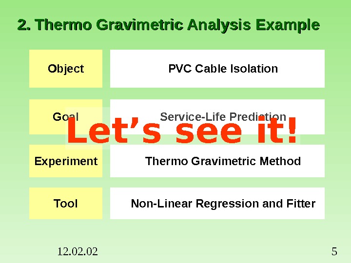
12. 02 52. Thermo Gravimetric Analysis Example Object PVC Cable Isolation Goal Service-Life Prediction Experiment Thermo Gravimetric Method Tool Non-Linear Regression and Fitter. Let’s see it!

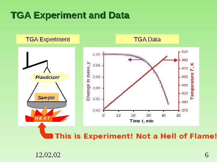
12. 02 6 TGA Experiment and Data Sam ple H E A T Plasticizer. TGA Experiment TGA Data This is Experiment! Not a Hell of Flame! 0. 900. 920. 940. 960. 981. 00 0 10 20 30 40 50 T ime t, min C ham ge in m ass, y 370390410430450470490510 Tem perature T , K

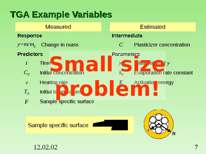
12. 02 7 TGA Example Variables Measured Estimated Response Intermediate y=m/m 0 Change in mass C Plasticizer concentration Predictors Parameters t Time y 0 Initial value of y C 0 Initial concentration k 0 Evaporation rate constant v Heating rate E Activation energy T 0 Initial temperature F Sample specific surface Rr. Sample specific surface 22 r. R R 2 V SF Small size problem!

12. 02 8 Plasticizer Evaporation Model Evaporation Law Volume Change The Arrhenius law Temperature growth T=T 0+vt y C 1 1 C 0 RT E k. Fk 0 exp 0 y 0 y. Ck dtdy )(, Diffusion is not relevant!

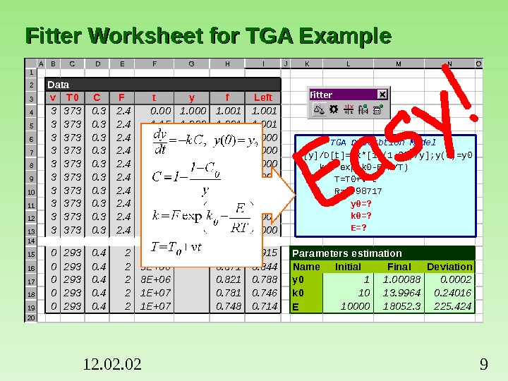
12. 02 9 A B C D E F G H I J K L M N O 1 2 Data 3 v T 0 C F t y f Left 4 3 373 0. 3 2. 4 0. 00 1. 001 5 3 373 0. 3 2. 4 1. 15 1. 000 1. 001 6 3 373 0. 3 2. 4 2. 25 1. 000 1. 001 1. 000 7 3 373 0. 3 2. 4 3. 40 1. 001 1. 000 8 3 373 0. 3 2. 4 4. 55 1. 000 1. 001 1. 000 9 3 373 0. 3 2. 4 5. 65 1. 000 1. 001 1. 000 10 3 373 0. 3 2. 4 6. 75 1. 000 1. 001 1. 000 11 3 373 0. 3 2. 4 7. 85 1. 000 12 3 373 0. 3 2. 4 9. 00 1. 000 13 3 373 0. 3 2. 4 10. 10 1. 000 14 15 0 293 0. 4 2 3 E+06 0. 931 0. 915 Parameters estimation 16 0 293 0. 4 2 5 E+06 0. 871 0. 844 Name Initial Final Deviation 17 0 293 0. 4 2 8 E+06 0. 821 0. 788 y 0 1 1. 00088 0. 0002 18 0 293 0. 4 2 1 E+07 0. 781 0. 746 k 0 10 13. 9964 0. 24016 19 0 293 0. 4 2 1 E+07 0. 748 0. 714 E 10000 18052. 3 225. 424 20 ‘TGA Desorbtion Model D[y]/D[t]=-k*[1 -(1 -C 0)/y]; y(0)=y 0 k=F*exp(k 0 -E/R/T) T=T 0+v*t R=1. 98717 y 0=? k 0=? E=? Fitter Worksheet for TGA Example

12. 02 10 Service Life Prediction by TGA Data

12. 02 113. NLR Basics

12. 02 12 Data and Errors Response Predictors Weights Parameters Fit Absolute error Weight and variance Relative erroriiify )(iii 1 fy. Const), cov( 2 ii 2 iw y 1 y 2. . y N y x 11 x 12. x 1 m x 21 x 22. x 2 m. . . . x N 1 x. N 2. x. Nm. X a 1 a 2. apa f 1 f 2. . . f Nf w 1 w 2. . . w N w. Weight is an effective instrument !

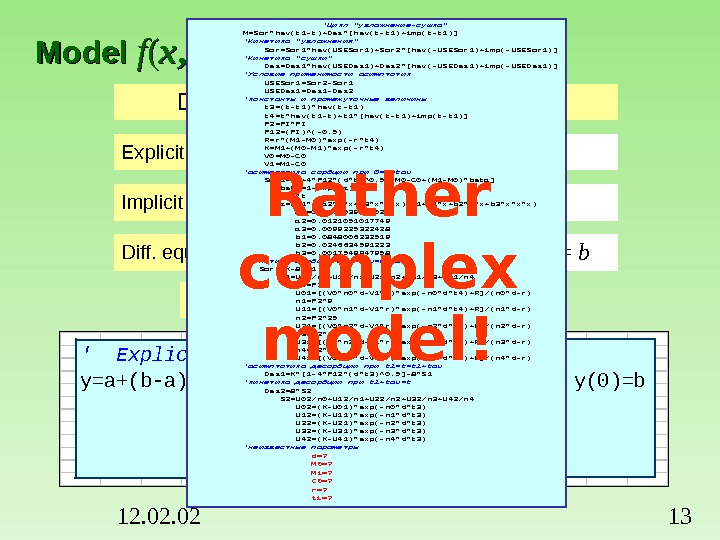
12. 02 13 Model ff (( xx , , aa )) Different shapes of the same model Explicit model y = a + ( b – a ) * exp( –c * x ) Implicit model 0 = a + ( b – a ) * exp( –c * x ) – y Diff. equation d[ y ]/d[ x ] = – c * ( y –a ); y ( 0 ) = b Presentation at worksheet’ Explicit model y=a+(b-a)*exp(-c*t) a=? b=? c=? ‘ Diff. equation d[y]/d[t]=-c*(y-a); y(0)=b a=? b=? c=? ‘Цикл «увлажнение-сушка»M=Sor*hev(t 1 -t)+Des*[hev(t-t 1)+imp(t-t 1)]’Кинетика «увлажнения» Sor=Sor 1*hev(USESor 1)+Sor 2*[hev(-USESor 1)+imp(-USESor 1)]’Кинетика «сушки» Des=Des 1*hev(USEDes 1)+Des 2*[hev(-USEDes 1)+imp(-USEDes 1)]’Условие применимости асимптотик USESor 1=Sor 2 -Sor 1 USEDes 1=Des 1 -Des 2’константы и промежуточные величины t 3=(t-t 1)*hev(t-t 1) t 4=t*hev(t 1 -t)+t 1*[hev(t-t 1)+imp(t-t 1)] P 2=PI*PI P 12=(PI)^(-0. 5) R=r*(M 1 -M 0)*exp(-r*t 4) K=M 1+(M 0 -M 1)*exp(-r*t 4) V 0=M 0 -C 0 V 1=M 1 -C 0’асимптотика сорбции при 0<t<tau Sor 1=C 0+4*P 12*(d*t)^0. 5*[M 0 -C 0+(M 1 -M 0)*beta] beta=1 -exp(-z) x=r*t z=(a 1*x+a 2*x*x+a 3*x*x*x)/(1+b 1*x+b 2*x*x+b 3*x*x*x) a 1=0. 6666539250029 a 2=0. 0121051017749 a 3=0. 0099225322428 b 1=0. 0848006232519 b 2=0. 0246634591223 b 3=0. 0017549947958'кинетика сорбции при tau<t<t 1 Sor 2=K-8*S 1 S 1=U 01/n 0+U 11/n 1+U 21/n 2+U 31/n 3+U 41/n 4 n 0=P 2 U 01=[(V 0*n 0*d-V 1*r)*exp(-n 0*d*t 4)+R]/(n 0*d-r) n 1=P 2*9 U 11=[(V 0*n 1*d-V 1*r)*exp(-n 1*d*t 4)+R]/(n 1*d-r) n 2=P 2*25 U 21=[(V 0*n 2*d-V 1*r)*exp(-n 2*d*t 4)+R]/(n 2*d-r) n 3=P 2*49 U 31=[(V 0*n 3*d-V 1*r)*exp(-n 3*d*t 4)+R]/(n 3*d-r) n 4=P 2*81 U 41=[(V 0*n 4*d-V 1*r)*exp(-n 4*d*t 4)+R]/(n 4*d-r)'асимптотика десорбции при t 1<t<t 1+tau Des 1=K*[1 -4*P 12*(d*t 3)^0. 5]-8*S 1'кинетика десорбции при t 1+tau<t Des 2=8*S 2 S 2=U 02/n 0+U 12/n 1+U 22/n 2+U 32/n 3+U 42/n 4 U 02=(K-U 01)*exp(-n 0*d*t 3) U 12=(K-U 11)*exp(-n 1*d*t 3) U 22=(K-U 21)*exp(-n 2*d*t 3) U 32=(K-U 31)*exp(-n 3*d*t 3) U 42=(K-U 41)*exp(-n 4*d*t 3)'неизвестные параметры d=? M 0=? M 1=? C 0=? r=? t 1=? Rather complex model!

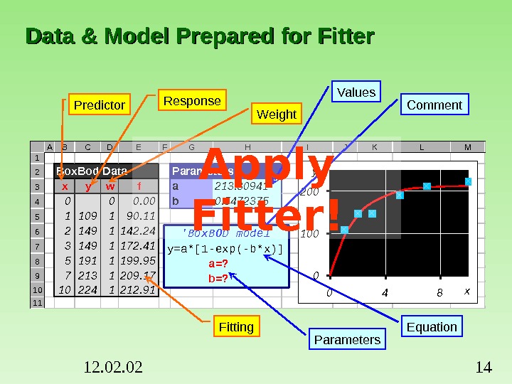
12. 02 14 A B C D E F G H I J K L M 1 2 3 4 5 6 7 8 9 10 11 A B C D E F G H I J K L M 1 2 Box. Bod Data 3 xywf 4 00 5 11091 6 21491 7 31491 8 51911 9 72131 10 102241 11 Data & Model Prepared for Fitter A B C D E F G H I J K L M 1 2 Box. Bod Data. Parameters 3 xywfa 100 4 00 b 0. 4 5 11091 6 21491 7 31491 8 51911 9 72131 10 102241 11 ‘Box. BOD model y=a*[1 -exp(-b*x)] a=? b=? A B C D E F G H I J K L M 1 2 Box. Bod Data Parameters 3 x y w f a 213. 80941 4 0 0 0. 00 b 0. 5472375 5 1 109 1 90. 11 6 2 149 1 142. 24 7 3 149 1 172. 41 8 5 191 1 199. 95 9 7 213 1 209. 17 10 10 224 1 212. 91 11 0100200 0 4 8 xy ‘Box. BOD model y=a*[1 -exp(-b*x)] a=? b=? Response Weight Fitting. Predictor Parameters Equation. Comment. Values Apply Fitter!

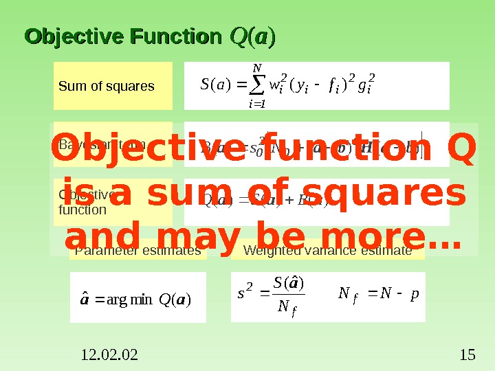
12. 02 15 Objective Function QQ (( aa )) Sum of squares Bayesian term Objective function N 1 i 2 ii 2 igfywa. S)()()(ba. Hbaa t 0 2 0 Ns. B )(min argˆaa. Q )()()(aaa. BSQ Parameter estimates p. NN N S sf f 2 )ˆ(a Weighted variance estimate. Objective function Q is a sum of squares and may be more…

12. 02 16 Very Important Matrix AA Hesse’s matrix Gauss’ approximation Model derivatives Covariance matrix F-matrix 112 s FACN 1 ip 1 a f w. V i ii, . . , ; , . . . , , ), ( ax p 1 aa Q 2 1 A 2 , , )( a 12 s CAF )regression linear in (XXVVA tt Matrix A is the cause of troubles. .

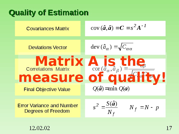
12. 02 17 Quality of Estimation Covariances Matrix Deviations Vector Correlations Matrix Final Objective Value Error Variance and Number Degrees of Freedom 12 s ACaa)ˆ, ˆ(cov CC C aa)ˆ, ˆ(cor Ca)ˆ(dev p. NN N ˆS sf f 2 )(a )(n im)ˆ(aa. QQMatrix A is the measure of quality!

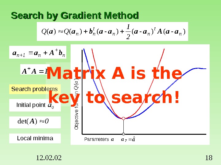
12. 02 18 Search by Gradient Method)-()-()-()()(n t nn 2 1 QQaa. Aaaaabaa Search problems Initial point a 0 Local minima 0)det(A nn 1 n b. Aaa IAA a 0 Parameters a O bjective function Q (a ) a 1 Parameters a O bjective function Q (a ) a 2 Parameters a O bjective function Q (a ) a 3 Parameters a O bjective function Q (a ) a 4 Parameters a O bjective function Q (a ) a 5 Parameters a O bjective function Q (a ) a 6 Parameters a O bjective function Q (a ) a 7 Parameters a O bjective function Q (a ) aˆMatrix A is the key to search!

12. 02 194. Multicollinearity

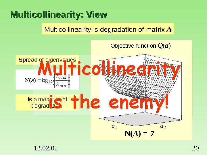
12. 02 20 Multicollinearity: View Multicollinearity is degradation of matrix A 00. 81. 62. 43. 244. 85. 66. 47. 28 01. 22. 43. 64. 867. 2 a 1 a 2 Objective function Q ( a ) 00. 81. 62. 43. 244. 85. 66. 47. 28 01. 22. 43. 64. 867. 2 a 1 a 2 Spread of eigenvalues is a measure of degradation min max 10 log)N( A 1 N( A ) =

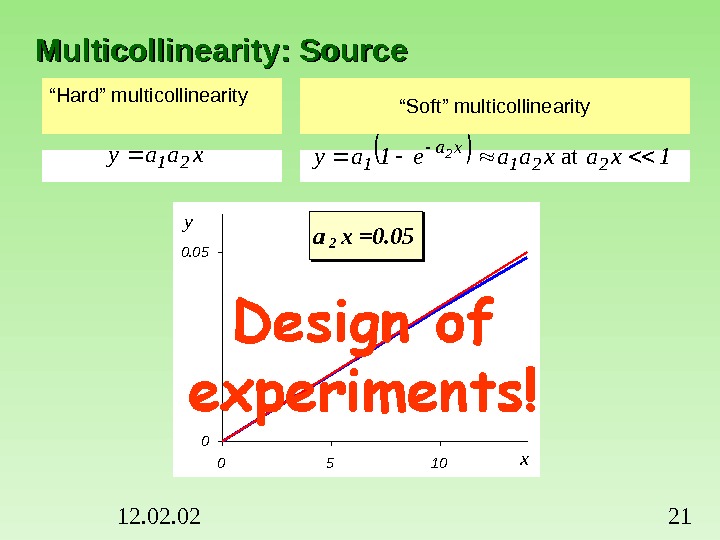
12. 02 21 a 2 x =1. 0 00. 8 0 5 10 xy a 2 x =0. 5 00. 4 0 5 10 xy. Multicollinearity: Source “ Hard” multicollinearity “ Soft” multicollinearityxaay 211 xaxaae 1 ay 221 xa 1 2 at a 2 x =0. 1 0 5 10 xy a 2 x =0. 05 0 5 10 xy

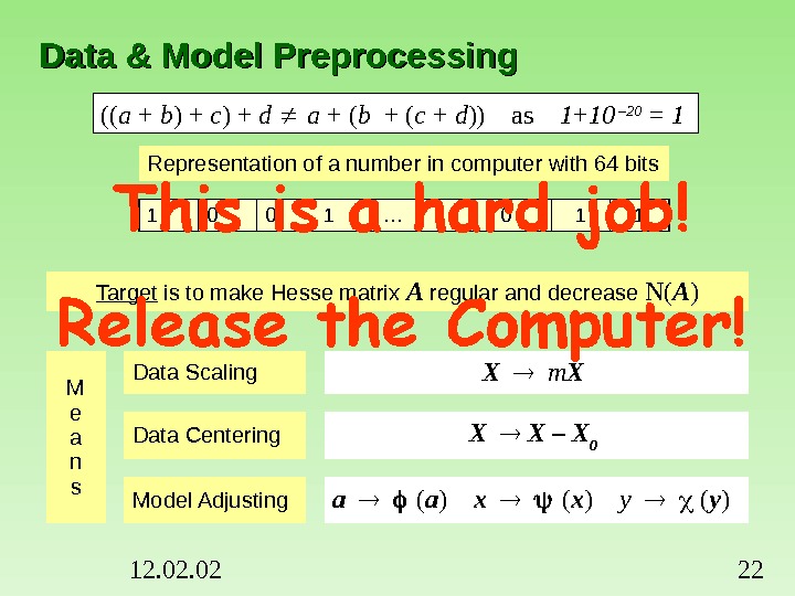
12. 02 22 Data & Model Preprocessing (( a + b ) + c ) + d a + ( b + ( c + d )) as 1 + 10 – 20 = 1 Representation of a number in computer with 64 bits 1 0 0 1 … 0 1 1 Target is to make Hesse matrix A regular and decrease N( A ) M e a n s Data Scaling X m X Data Centering X X – X 0 Model Adjusting a ( a ) x ( x ) y ( y )

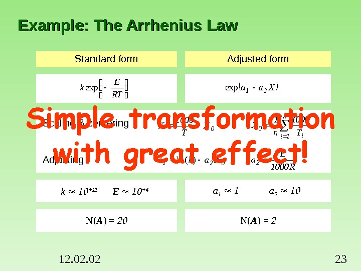
12. 02 23 Example: The Arrhenius Law Standard form Adjusted form Scaling & centering Adjusting k 10 +11 E 10 +4 a 1 1 a 2 10 N( A ) = 20 N( A ) = 2 Xaa 21 exp R 1000 E a 2021 Xaka)(ln n 1 ii 0 T 1000 n 1 X 0 X T 1000 X RT E kexp

12. 02 24 Derivative Calculation and Precision N( A ) A -1 y=f ( a, x ) 0=f ( y , a, x ) dy/dx=f ( y , a, x ) 6 6+2=8 8+0=8 8+2=10 10+2=128 8+2=10 10+0=10 10+2=12 12+2=1410 10+2=12 12+0=12 12+2=14 14+2=16 2) Auto calculation of analytical derivatives f=exp(-a*t) df/da=-t*exp(-a*t)h afhaf a f)()( 1) Numerical calculation of difference derivatives

12. 02 255. Prediction

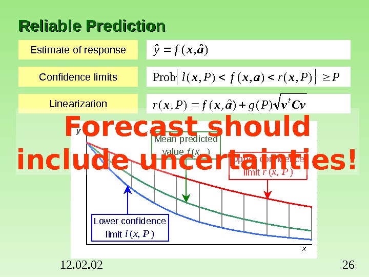
12. 02 26 Reliable Predictiony x Upper confidence limit r(x, P) Lower confidence limit l(x, P) Mean predicted value f(x, ) a ˆEstimate of response Confidence limits Linearization )ˆ, (ˆaxfy Cvvaxx t Pgf. Pr)()ˆ, (), ( PPrf. Pl), (), (Probxaxx Forecast should include uncertainties!

12. 02 27 Nonlinearity and Simulation)(, , ), ˆ(~ * xaa. Caa **** P, rff. NM 1 M 1 a 1 a 2 Objective’s Contour )()ˆ ()( Ps. QQ 2 p 2 aa Approximating Ellipse )()ˆ ( Ps 2 p 2 t aa. Aaa a ˆNon-linear models call for special methods of reliable prediction!

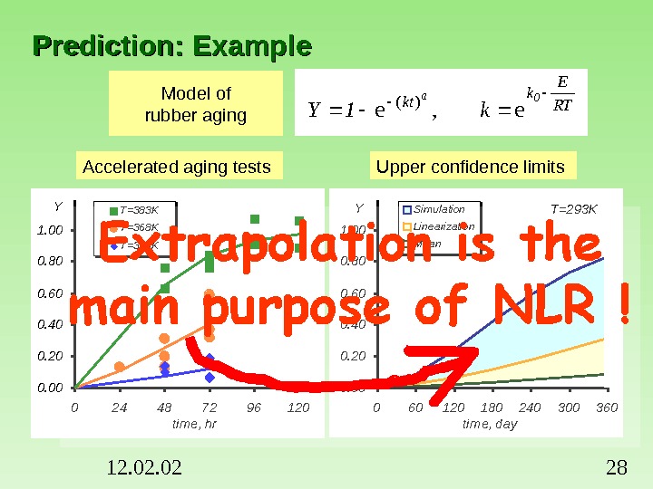
12. 02 28 Prediction: Example 0. 000. 200. 400. 600. 801. 00 0 24 48 72 96 120 tim e, hr. Y T=383 K T=368 K T=353 K T=293 K 0. 000. 200. 400. 600. 801. 00 0 60 120 180 240 300 360 tim e, day. Y Simulation Linearization Mean. Accelerated aging tests Upper confidence limits. Model of rubber aging RT E k kt 0 ak 1 Y ee, )(

12. 02 296. Testing

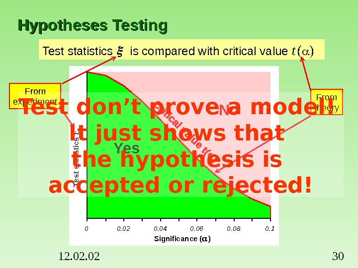
12. 02 30 Hypotheses Testing Test statistics is compared with critical value t ( ) No Yes 0 0. 02 0. 04 0. 06 0. 08 0. 1 Significance ( ) Test statistics From theory. From experiment Test don’t prove a model! It just shows that the hypothesis is accepted or rejected!

12. 02 31 Lack-of-Fit and Variances Tests These hypotheses are based on variances and they can’t be tested without replicas ! 0255075100 0. 5 1. 5 2. 5 3. 5 4. 5 5. 5 Predictor. R esponse 0246 Variance Replica 1 Variances by replicas. Replica 2 Lack-of-Fit is a wily test!

12. 02 32 Series of signs 5 Positive residuals 6 Negative residuals 11 Outlier 0. 2 0. 4 0. 6 0. 8 1 1. 2 051015 Predictor R esponse. Outlier and Series Tests These hypotheses are based on residuals and they can be tested without replicas Positive residual Negative residual Acceptable deviation Series test is very sensitive!

12. 02 337. Bayesian Estimation

12. 02 34 Bayesian Estimation y 1 X 1 y 2 X 2. . . y k X k. . . f 1 ( X 1 , a 0 , a 1 ) f 2 ( X 2 , a 0 , a 2 ) f k ( X k , a 0 , a k )Data set 1 Data set 2 Data set k Post a 0 , a 1 s 1 2 N 1 Prior a 0 s 1 2 N 1 Post a 0 , a 2 s 2 2 N 2 Prior a 0 s k 2 N k Post a 0 , a k s k 2 N k Result a 0 , a 1 , …, a k s 2 NHow to eat away an elephant? Slice by slice!

12. 02 35 Posterior and Prior Information. Type I Posterior Information Parameter estimates Prior parameter values b Matrix F Recalculated matrix H Error variance s 2 Prior variance value s 0 2 NDF N f Prior NDF N 0 Objective Functionaˆ )()()( ba. Hbaaaa a. Baa t 0 2 0 RRNs. B SQThe same error in each portion of data!

12. 02 36 Posterior and Prior Information. Type II Posterior Information Parameter estimates Prior parameter values b Matrix F Recalculated matrix H Objective Functionaˆ )()()( )( exp)( )()()( ba. Hbaa a a a. Baa t R N R B SQ Different errors in each portion of data!

12. 02 378. Conclusions Mysterious Nature LR Model NLR Model Thank you!