Predictive Indicators MESA Software John Ehlers e-mail ehlers mesasoftware

Predictive Indicators MESA Software John Ehlers e-mail: ehlers@mesasoftware. com SLIDE 1

AGENDA n SLIDE 2 Exponential Moving Averages • Why lag is important • How to compute the EMA constant to produce a given lag n Higher order filters • Let your computer do a superior job of smoothing n n n Essence of Predictive Filters Linear Kalman Filters Nonlinear Kalman Filters Theoretically Optimum Predictive Filters Zero Lag smoothing

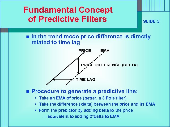Fundamental Concept of Predictive Filters SLIDE 3 n In the trend mode price difference is directly related to time lag n Procedure to generate a predictive line: • Take an EMA of price (better, a 3 Pole filter) • Take the difference ( delta) between the price and its EMA • Form the predictor by adding delta to the price – equivalent to adding 2*delta to EMA

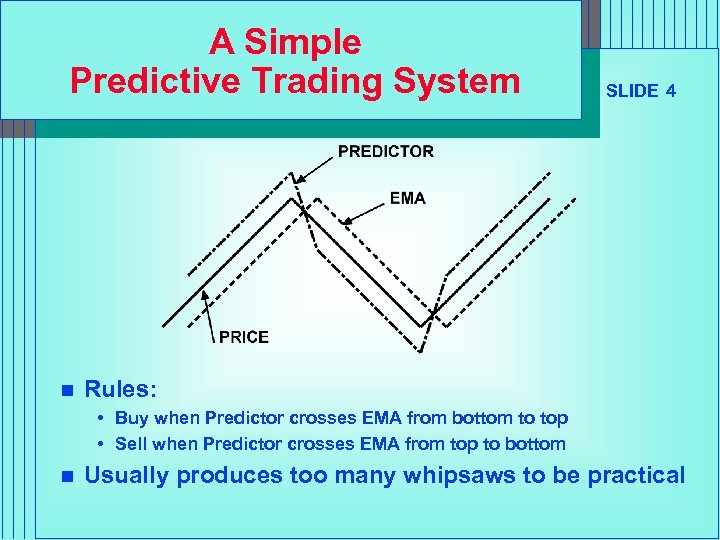A Simple Predictive Trading System n SLIDE 4 Rules: • Buy when Predictor crosses EMA from bottom to top • Sell when Predictor crosses EMA from top to bottom n Usually produces too many whipsaws to be practical

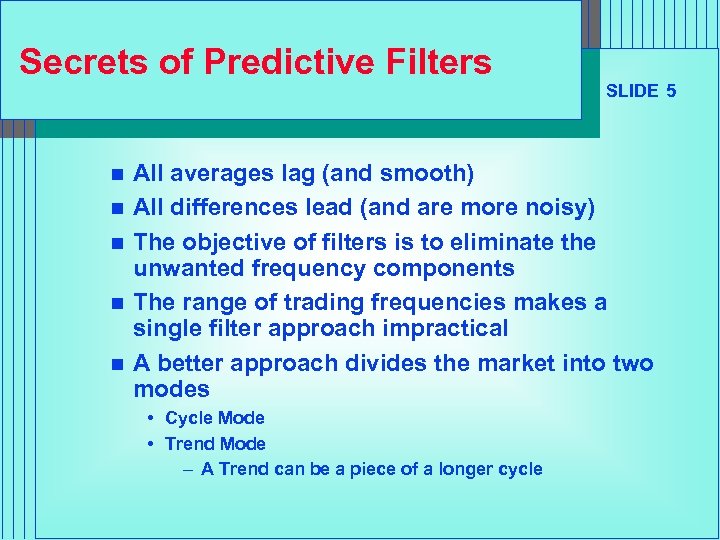Secrets of Predictive Filters n n n SLIDE 5 All averages lag (and smooth) All differences lead (and are more noisy) The objective of filters is to eliminate the unwanted frequency components The range of trading frequencies makes a single filter approach impractical A better approach divides the market into two modes • Cycle Mode • Trend Mode – A Trend can be a piece of a longer cycle

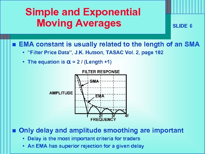Simple and Exponential Moving Averages n SLIDE 6 EMA constant is usually related to the length of an SMA • “Filter Price Data”, J. K. Hutson, TASAC Vol. 2, page 102 • The equation is a = 2 / (Length +1) n Only delay and amplitude smoothing are important • Delay is the most important criteria for traders • An EMA has superior rejection for a given delay

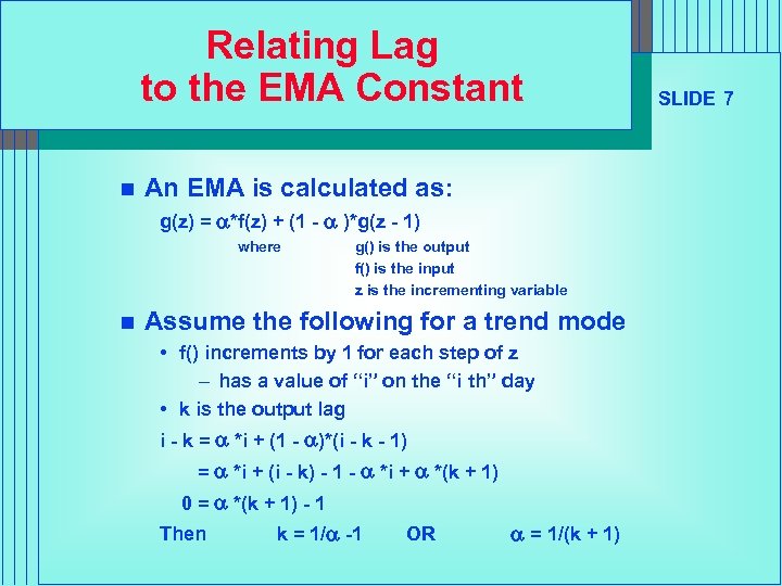Relating Lag to the EMA Constant n An EMA is calculated as: g(z) = a*f(z) + (1 - a )*g(z - 1) where n g() is the output f() is the input z is the incrementing variable Assume the following for a trend mode • f() increments by 1 for each step of z – has a value of “i” on the “i th” day • k is the output lag i - k = a *i + (1 - a)*(i - k - 1) = a *i + (i - k) - 1 - a *i + a *(k + 1) 0 = a *(k + 1) - 1 Then k = 1/a -1 OR a = 1/(k + 1) SLIDE 7

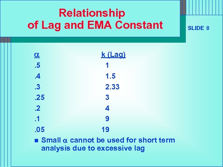Relationship of Lag and EMA Constant a k (Lag). 5 1. 4 1. 5. 3 2. 33. 25 3. 2 4. 1 9. 05 19 n Small a cannot be used for short term analysis due to excessive lag SLIDE 8

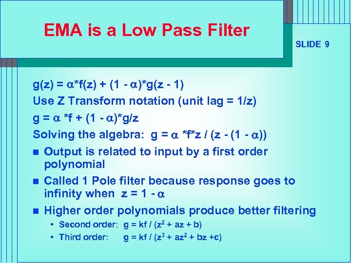EMA is a Low Pass Filter SLIDE 9 g(z) = a*f(z) + (1 - a)*g(z - 1) Use Z Transform notation (unit lag = 1/z) g = a *f + (1 - a)*g/z Solving the algebra: g = a *f*z / (z - (1 - a)) n Output is related to input by a first order polynomial n Called 1 Pole filter because response goes to infinity when z = 1 - a n Higher order polynomials produce better filtering • Second order: g = kf / (z 2 + az + b) • Third order: g = kf / (z 3 + az 2 + bz +c)

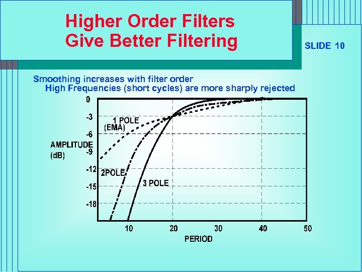Higher Order Filters Give Better Filtering Smoothing increases with filter order High Frequencies (short cycles) are more sharply rejected SLIDE 10

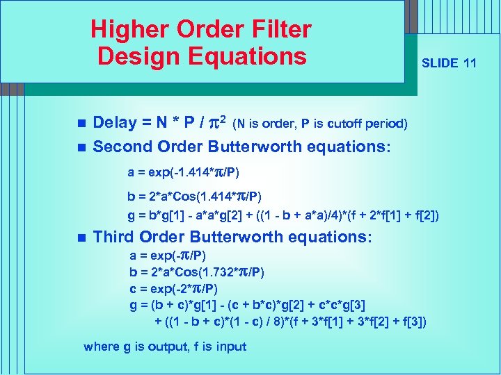Higher Order Filter Design Equations n n SLIDE 11 Delay = N * P / p 2 (N is order, P is cutoff period) Second Order Butterworth equations: a = exp(-1. 414*p/P) b = 2*a*Cos(1. 414*p/P) g = b*g[1] - a*a*g[2] + ((1 - b + a*a)/4)*(f + 2*f[1] + f[2]) n Third Order Butterworth equations: a = exp(-p/P) b = 2*a*Cos(1. 732*p/P) c = exp(-2*p/P) g = (b + c)*g[1] - (c + b*c)*g[2] + c*c*g[3] + ((1 - b + c)*(1 - c) / 8)*(f + 3*f[1] + 3*f[2] + f[3]) where g is output, f is input

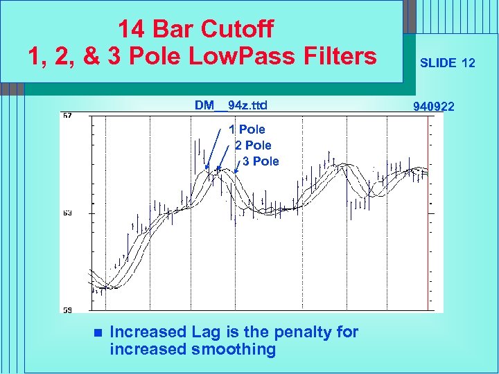14 Bar Cutoff 1, 2, & 3 Pole Low. Pass Filters DM__94 z. ttd 1 Pole 2 Pole 3 Pole n Increased Lag is the penalty for increased smoothing SLIDE 12 940922

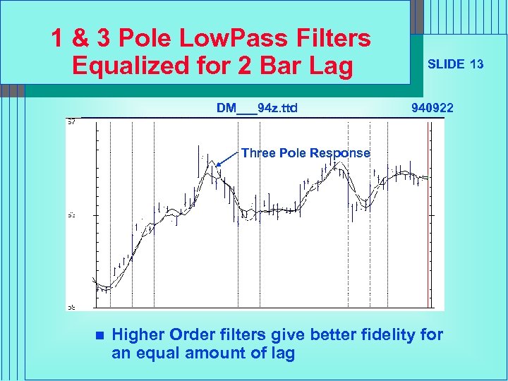1 & 3 Pole Low. Pass Filters Equalized for 2 Bar Lag DM___94 z. ttd SLIDE 13 940922 Three Pole Response n Higher Order filters give better fidelity for an equal amount of lag

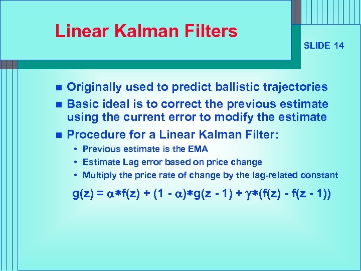Linear Kalman Filters n n n SLIDE 14 Originally used to predict ballistic trajectories Basic ideal is to correct the previous estimate using the current error to modify the estimate Procedure for a Linear Kalman Filter: • Previous estimate is the EMA • Estimate Lag error based on price change • Multiply the price rate of change by the lag-related constant g(z) = a*f(z) + (1 - a)*g(z - 1) + g*(f(z) - f(z - 1))

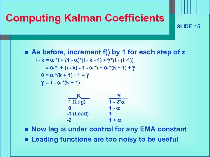Computing Kalman Coefficients n As before, increment f() by 1 for each step of z i - k = a *i + (1 - a)*(i - k - 1) + g*(i -1)) = a *i + (i - k) - 1 - a *i + a *(k + 1) + g 0 = a *(k + 1) - 1 + g g = 1 - a *(k + 1) ___K___ 1 (Lag) 0 -1 (Lead) -2 n n SLIDE 15 ___g__ 1 - 2*a 1 -a 1 1+a Now lag is under control for any EMA constant Leading functions are too noisy to be useful

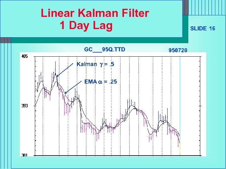Linear Kalman Filter 1 Day Lag GC___95 Q. TTD Kalman g =. 5 EMA a =. 25 SLIDE 16 950728

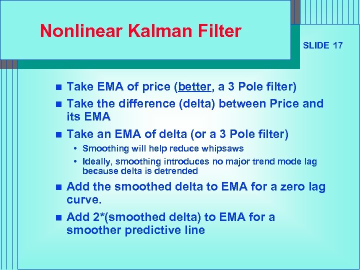Nonlinear Kalman Filter n n n SLIDE 17 Take EMA of price (better, a 3 Pole filter) Take the difference (delta) between Price and its EMA Take an EMA of delta (or a 3 Pole filter) • Smoothing will help reduce whipsaws • Ideally, smoothing introduces no major trend mode lag because delta is detrended n n Add the smoothed delta to EMA for a zero lag curve. Add 2*(smoothed delta) to EMA for a smoother predictive line

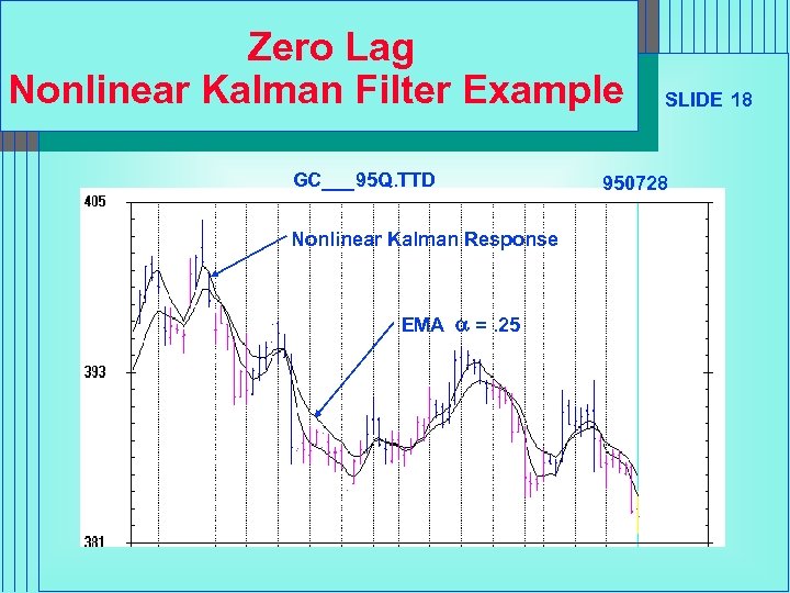Zero Lag Nonlinear Kalman Filter Example GC___95 Q. TTD Nonlinear Kalman Response EMA a =. 25 SLIDE 18 950728

Theoretically Optimum Predictive Filters n SLIDE 19 Optimum predictive filters are solutions to the generalized Wiener-Hopf integral equation • “Statistical Theory of Communication”, Y. W. Lee, John Wiley and Sons, 1960 n n Optimum Predictive filters pertain only to the market cycle mode (Must use detrended waveforms) Two solutions are of interest to traders • Pure predictor (noise free case) – See “The Band. Pass Indicator”, John Ehlers, TASAC, September 1994, page 51 • Predicting in the presence of noise – See “Optimum Predictive Filters”, John Ehlers, TASAC, June 1995, Page 38

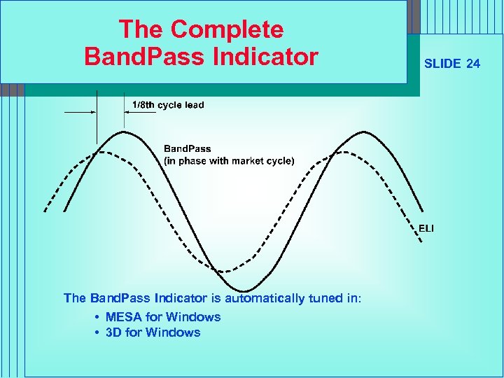
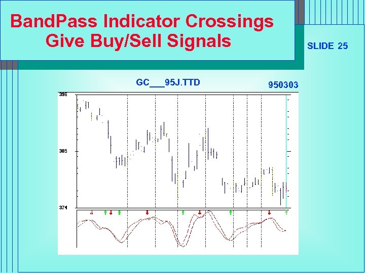
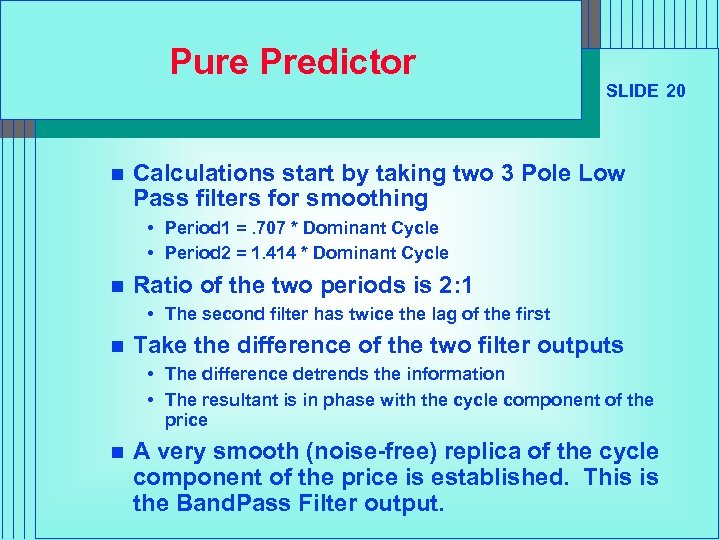Pure Predictor n SLIDE 20 Calculations start by taking two 3 Pole Low Pass filters for smoothing • Period 1 =. 707 * Dominant Cycle • Period 2 = 1. 414 * Dominant Cycle n Ratio of the two periods is 2: 1 • The second filter has twice the lag of the first n Take the difference of the two filter outputs • The difference detrends the information • The resultant is in phase with the cycle component of the price n A very smooth (noise-free) replica of the cycle component of the price is established. This is the Band. Pass Filter output.

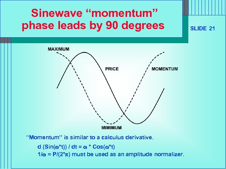Sinewave “momentum” phase leads by 90 degrees “Momentum” is similar to a calculus derivative. d (Sin(w*t)) / dt = w * Cos(w*t) 1/w = P/(2*p) must be used as an amplitude normalizer. SLIDE 21

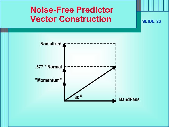
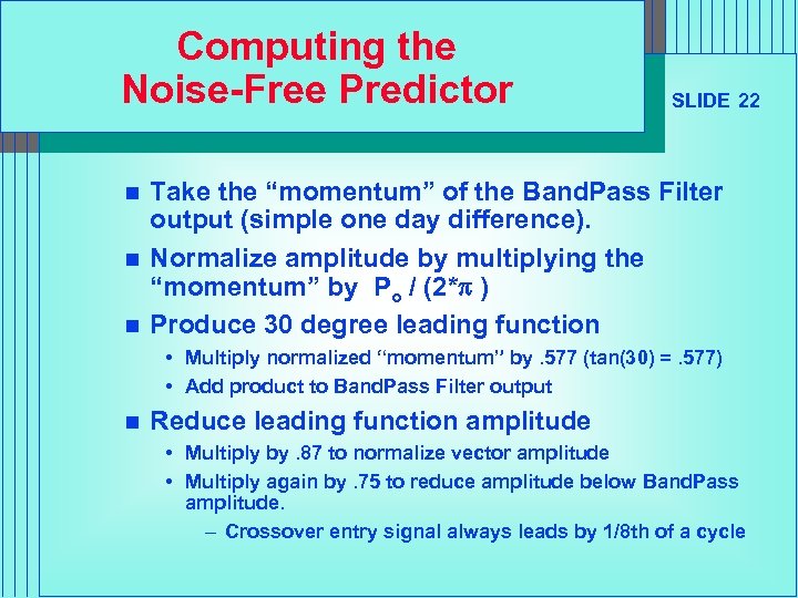Computing the Noise-Free Predictor n n n SLIDE 22 Take the “momentum” of the Band. Pass Filter output (simple one day difference). Normalize amplitude by multiplying the “momentum” by Po / (2*p ) Produce 30 degree leading function • Multiply normalized “momentum” by. 577 (tan(30) =. 577) • Add product to Band. Pass Filter output n Reduce leading function amplitude • Multiply by. 87 to normalize vector amplitude • Multiply again by. 75 to reduce amplitude below Band. Pass amplitude. – Crossover entry signal always leads by 1/8 th of a cycle

Noise-Free Predictor Vector Construction SLIDE 23

The Complete Band. Pass Indicator The Band. Pass Indicator is automatically tuned in: • MESA for Windows • 3 D for Windows SLIDE 24

Band. Pass Indicator Crossings Give Buy/Sell Signals GC___95 J. TTD 950303 SLIDE 25

Optimum Predictive Filter in the Presence of Noise n SLIDE 26 Start with RSI or Stochastic Indicator • Provides detrended waveform • Adjust length until the waveform resembles a sinewave n Technique is useful only when the waveform has a Poisson probability distribution • The midpoint crossings must be relatively regular n Take an EMA of the RSI • a =. 25 is nominally correct (gives a 3 day lag) n Subtract the EMA from the RSI to produce the predictor • Remember the fundamental premise in constructing predictive filters?

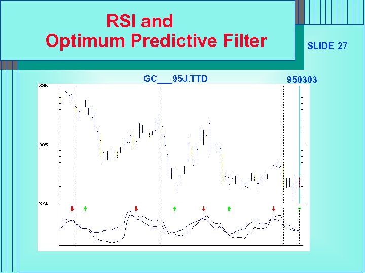RSI and Optimum Predictive Filter GC___95 J. TTD SLIDE 27 950303

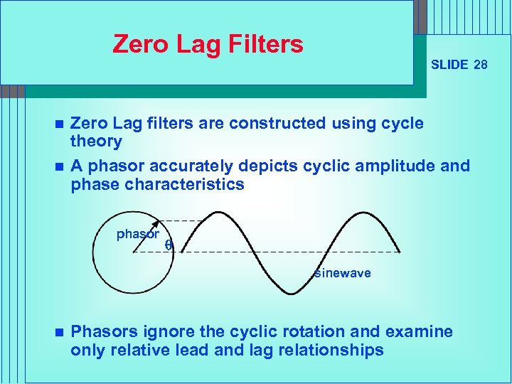Zero Lag Filters n n SLIDE 28 Zero Lag filters are constructed using cycle theory A phasor accurately depicts cyclic amplitude and phase characteristics phasor q sinewave n Phasors ignore the cyclic rotation and examine only relative lead and lag relationships

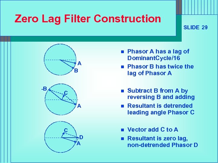Zero Lag Filter Construction n A B -B n n C A C n n D A n SLIDE 29 Phasor A has a lag of Dominant. Cycle/16 Phasor B has twice the lag of Phasor A Subtract B from A by reversing B and adding Resultant is detrended leading angle Phasor C Vector add C to A Resultant is zero lag, non-detrended Phasor D

Zero Lag Filter Example GC___95 Q. TTD SLIDE 30 950728

A Zero Lag Filter Application n SLIDE 31 Take a 3 Pole zero lag filter of price highs Take a 3 Pole zero lag filter of price lows Calculate statistics of the high and low variations • Add 2 Standard Deviations to the Highs Zero Lag Filter • Subtract 2 Standard Deviations to the Lows Zero Lag Filter n n n Resultant channels can be used as stop values for a stop-and-reverse system Remove the +/- Std Deviations near cycle turns SUMMIT for Windows uses this procedure

SUMMARY n SLIDE 32 What you have learned: • • How to relate filter lag to EMA constant How to compute Higher Order Butterworth Filters How to control lag using a Linear Kalman Filter How to compute a Nonlinear Kalman Filter – Possible start for a crossover system • How to compute Optimum Predictive Filters for the cycle mode – Pure Predictor (Noise-Free, using higher order filters) – With RSI or Stochastics • How to compute a zero lag filter