Modigliani Miller WACC FIN 591 Financial

Modigliani & Miller + WACC FIN 591: Financial Fundamentals/Valuation

M&M: The Starting Point n n n A number of restrictive assumptions apply Use the additivity principle Derive propositions re: valuation and cost of capital n Derived in both the “no tax” and “tax” cases. FIN 591: Financial Fundamentals/Valuation 2

The M&M Assumptions n n Homogeneous expectations Homogeneous business risk (s. EBIT) classes Perpetual no-growth cash flows Perfect capital markets: Perfect competition; i. e. , everyone is a price taker n Firms and investors borrow and lend at the same rate n Equal access to all relevant information n No transaction costs (no taxes or bankruptcy costs). n FIN 591: Financial Fundamentals/Valuation 3

Business Risk n Business risk: n n Risk surrounding expected operating cash flows Factors causing high business risk: n High correlation between the firm and the economy Firm has small market share in competitive market Firm is small relative to competitors Firm is not well diversified n Firm has high fixed operating costs. n n n FIN 591: Financial Fundamentals/Valuation 4

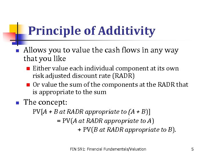Principle of Additivity n Allows you to value the cash flows in any way that you like Either value each individual component at its own risk adjusted discount rate (RADR) n Or value the sum of the components at the RADR that is appropriate to the sum n n The concept: PV[A + B at RADR appropriate to (A + B)] = PV(A at RADR appropriate to A) + PV(B at RADR appropriate to B). FIN 591: Financial Fundamentals/Valuation 5

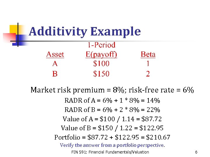Additivity Example Market risk premium = 8%; risk-free rate = 6% RADR of A = 6% + 1 * 8% = 14% RADR of B = 6% + 2 * 8% = 22% Value of A = $100 / 1. 14 = $87. 72 Value of B = $150 / 1. 22 = $122. 95 Portfolio = $87. 72 + $122. 95 = $210. 67 Verify the answer from a portfolio perspective. FIN 591: Financial Fundamentals/Valuation 6

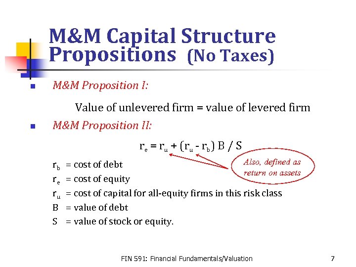M&M Capital Structure Propositions (No Taxes) n M&M Proposition I: n Value of unlevered firm = value of levered firm M&M Proposition II: re = ru + (ru - rb) B / S rb re ru B S Also, defined as = cost of debt return on assets = cost of equity = cost of capital for all-equity firms in this risk class = value of debt = value of stock or equity. FIN 591: Financial Fundamentals/Valuation 7

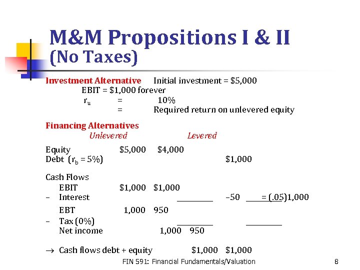M&M Propositions I & II (No Taxes) Investment Alternative Initial investment = $5, 000 EBIT = $1, 000 forever ru = 10% = Required return on unlevered equity Financing Alternatives Unlevered Equity Debt (rb = 5%) Cash Flows EBIT – Interest EBT – Tax (0%) Net income $5, 000 Levered $4, 000 $1, 000 – 50 = (. 05)1, 000 950 ® Cash flows debt + equity $1, 000 FIN 591: Financial Fundamentals/Valuation 8

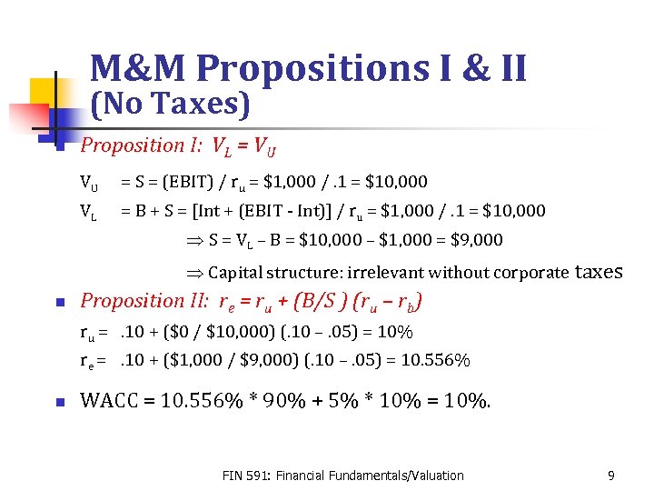M&M Propositions I & II (No Taxes) n Proposition I: VL = VU VU = S = (EBIT) / ru = $1, 000 /. 1 = $10, 000 VL = B + S = [Int + (EBIT - Int)] / ru = $1, 000 /. 1 = $10, 000 Þ S = VL – B = $10, 000 – $1, 000 = $9, 000 Þ Capital structure: irrelevant without corporate taxes n Proposition II: re = ru + (B/S ) (ru – rb) ru =. 10 + ($0 / $10, 000) (. 10 –. 05) = 10% re =. 10 + ($1, 000 / $9, 000) (. 10 –. 05) = 10. 556% n WACC = 10. 556% * 90% + 5% * 10% = 10%. FIN 591: Financial Fundamentals/Valuation 9

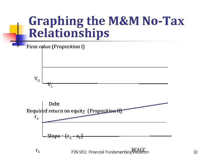Graphing the M&M No-Tax Relationships Firm value (Proposition I) VU VL Debt Required return on equity (Proposition II) re Slope = (ru – rb ) ru WACC FIN 591: Financial Fundamentals/Valuation 10

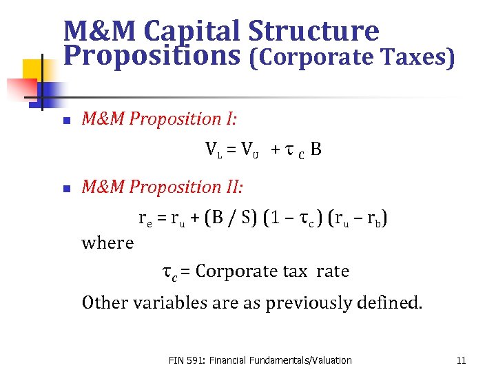M&M Capital Structure Propositions (Corporate Taxes) n M&M Proposition I: VL = V U + t C B n M&M Proposition II: re = ru + (B / S) (1 – tc ) (ru – rb) where tc = Corporate tax rate Other variables are as previously defined. FIN 591: Financial Fundamentals/Valuation 11

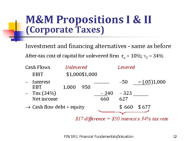M&M Propositions I & II (Corporate Taxes) Investment and financing alternatives - same as before After-tax cost of capital for unlevered firm ru = 10%; t. C = 34% Cash Flows EBIT – Interest EBT – Tax (34%) Net income Unlevered $1, 000 950 ® Cash flow debt + equity Levered – 50 – 340 660 = (. 05)1, 000 – 323 627 $ 660 $ 677 $17 difference = $50 interest x 34% tax rate FIN 591: Financial Fundamentals/Valuation 12

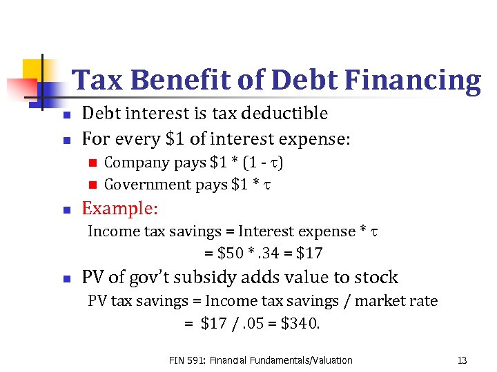Tax Benefit of Debt Financing n n Debt interest is tax deductible For every $1 of interest expense: Company pays $1 * (1 - t) n Government pays $1 * t n n Example: Income tax savings = Interest expense * t = $50 *. 34 = $17 n PV of gov’t subsidy adds value to stock PV tax savings = Income tax savings / market rate = $17 /. 05 = $340. FIN 591: Financial Fundamentals/Valuation 13

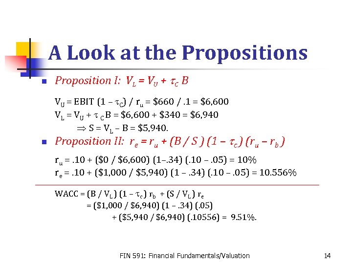A Look at the Propositions n Proposition I: VL = VU + t. C B VU = EBIT (1 – t. C) / ru = $660 /. 1 = $6, 600 VL = VU + t C B = $6, 600 + $340 = $6, 940 Þ S = VL – B = $5, 940. n Proposition II: re = ru + (B / S ) (1 – tc ) (ru – rb ) ru =. 10 + ($0 / $6, 600) (1–. 34) (. 10 –. 05) = 10% re =. 10 + ($1, 000 / $5, 940) (1 –. 34) (. 10 –. 05) = 10. 556% WACC = (B / VL ) (1 – tc ) rb + (S / VL ) re = ($1, 000 / $6, 940) (1 –. 34) (. 05) + ($5, 940 / $6, 940) (. 10556) = 9. 51%. FIN 591: Financial Fundamentals/Valuation 14

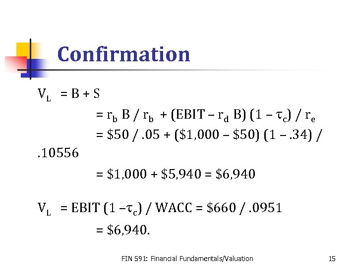Confirmation VL = B + S = rb B / rb + (EBIT – rd B) (1 – tc) / re = $50 /. 05 + ($1, 000 – $50) (1 –. 34) /. 10556 = $1, 000 + $5, 940 = $6, 940 VL = EBIT (1 –tc) / WACC = $660 /. 0951 = $6, 940. FIN 591: Financial Fundamentals/Valuation 15

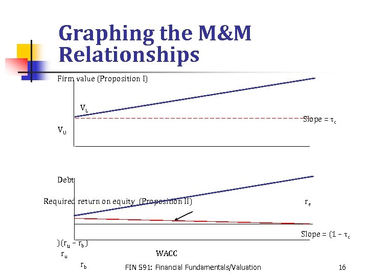Graphing the M&M Relationships Firm value (Proposition I) VL Slope = tc VU Debt Required return on equity (Proposition II) )(ru – rb ) ru rb re Slope = (1 – tc WACC FIN 591: Financial Fundamentals/Valuation 16

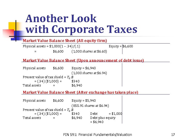Another Look with Corporate Taxes Market Value Balance Sheet (All equity firm) Physical assets = $1, 000(1 –. 34)/(. 1) Equity = $6, 600 (1, 000 shares at $6. 60) Market Value Balance Sheet (Upon announcement of debt issue) Physical assets $6, 600 Equity = $6, 940 (1, 000 shares at $6. 94) Present value of tax shield = TC B = (. 34) ($1, 000) = $340 Total assets = $6, 940 Market Value Balance Sheet (After exchange has taken place) Physical assets $6, 600 Equity = $5, 940 (855. 91 shares at $6. 94) Present value of tax shield = TC B = (. 34) ($1, 000) = $340 Debt = $1, 000 Total assets = $6, 940 Debt plus equity = $6, 940 FIN 591: Financial Fundamentals/Valuation 17

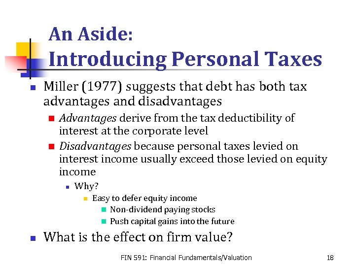An Aside: Introducing Personal Taxes n Miller (1977) suggests that debt has both tax advantages and disadvantages Advantages derive from the tax deductibility of interest at the corporate level n Disadvantages because personal taxes levied on interest income usually exceed those levied on equity income n n Why? n n Easy to defer equity income n Non-dividend paying stocks n Push capital gains into the future What is the effect on firm value? FIN 591: Financial Fundamentals/Valuation 18

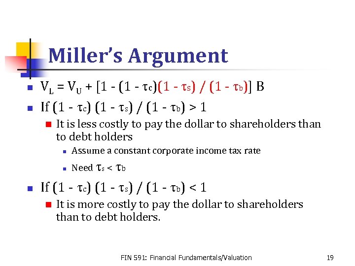Miller’s Argument n n VL = VU + [1 - (1 - tc)(1 - ts) / (1 - tb)] B If (1 - tc) (1 - ts) / (1 - tb) > 1 n It is less costly to pay the dollar to shareholders than to debt holders n tb If (1 - tc) (1 - ts) / (1 - tb) < 1 n n Assume a constant corporate income tax rate n Need ts < It is more costly to pay the dollar to shareholders than to debt holders. FIN 591: Financial Fundamentals/Valuation 19

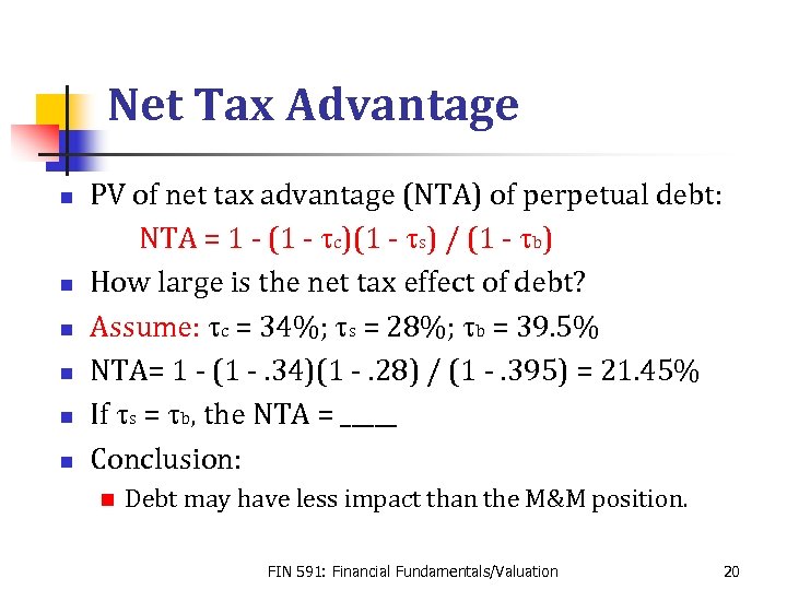Net Tax Advantage n n n PV of net tax advantage (NTA) of perpetual debt: NTA = 1 - (1 - tc)(1 - ts) / (1 - tb) How large is the net tax effect of debt? Assume: tc = 34%; ts = 28%; tb = 39. 5% NTA= 1 - (1 -. 34)(1 -. 28) / (1 -. 395) = 21. 45% If ts = tb, the NTA = _____ Conclusion: n Debt may have less impact than the M&M position. FIN 591: Financial Fundamentals/Valuation 20

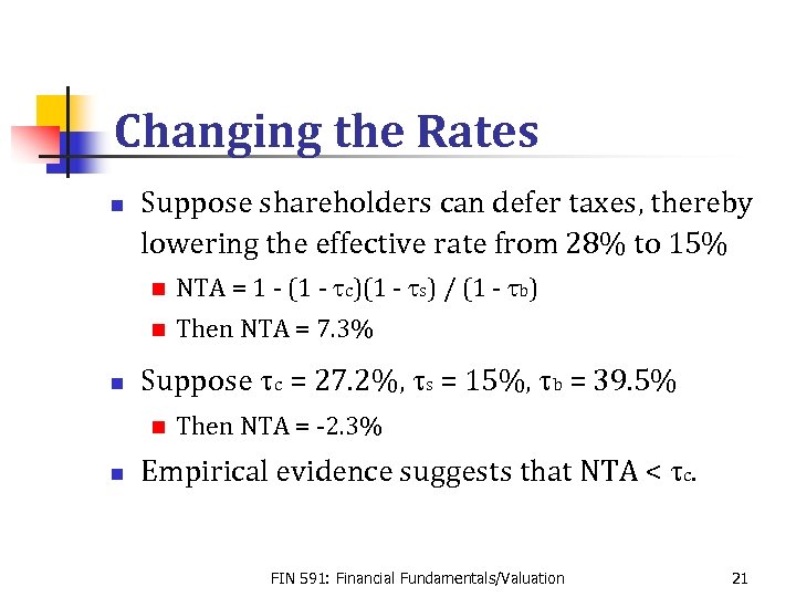Changing the Rates n Suppose shareholders can defer taxes, thereby lowering the effective rate from 28% to 15% n n n NTA = 1 - (1 - tc)(1 - ts) / (1 - tb) Then NTA = 7. 3% Suppose tc = 27. 2%, ts = 15%, tb = 39. 5% n n Then NTA = -2. 3% Empirical evidence suggests that NTA < tc. FIN 591: Financial Fundamentals/Valuation 21

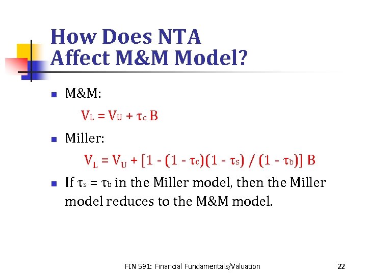How Does NTA Affect M&M Model? n M&M: VL = V U + t c B n Miller: VL = VU + [1 - (1 - tc)(1 - ts) / (1 - tb)] B n If ts = tb in the Miller model, then the Miller model reduces to the M&M model. FIN 591: Financial Fundamentals/Valuation 22

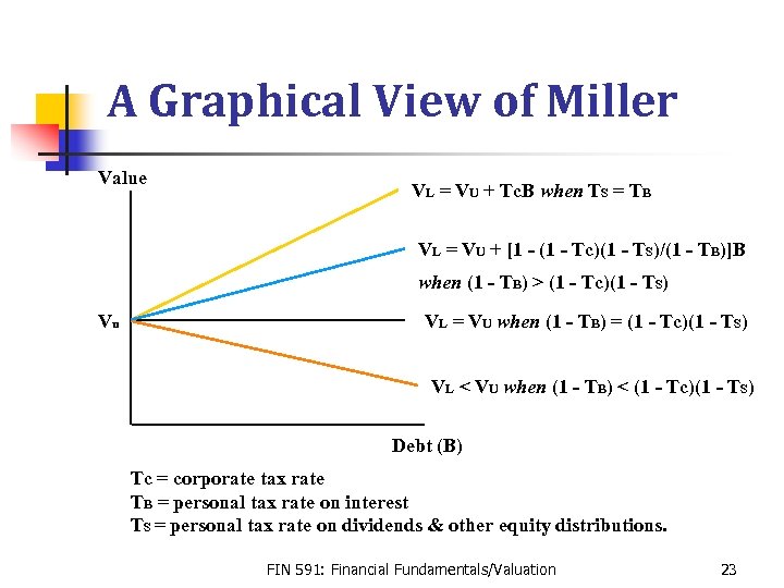A Graphical View of Miller Value VL = VU + Tc. B when TS = TB VL = VU + [1 - (1 - Tc)(1 - TS)/(1 - TB)]B when (1 - TB) > (1 - Tc)(1 - TS) Vu VL = VU when (1 - TB) = (1 - Tc)(1 - TS) VL < VU when (1 - TB) < (1 - Tc)(1 - TS) Debt (B) Tc = corporate tax rate TB = personal tax rate on interest TS = personal tax rate on dividends & other equity distributions. FIN 591: Financial Fundamentals/Valuation 23

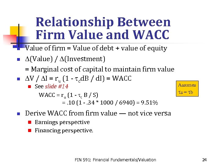Relationship Between Firm Value and WACC n n n Value of firm = Value of debt + value of equity D(Value) / D(Investment) = Marginal cost of capital to maintain firm value DV / DI = ru (1 - tcd. B / d. I) = WACC n n See slide #14 WACC = ru (1 - tc B / S) =. 10 (1 -. 34 * 1000 / 6940) = 9. 51% Assumes ts = tb Derive WACC from firm value — not vice versa Earnings perspective n Financing perspective. n FIN 591: Financial Fundamentals/Valuation 24

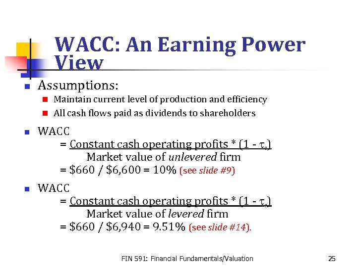WACC: An Earning Power View n Assumptions: Maintain current level of production and efficiency n All cash flows paid as dividends to shareholders n n n WACC = Constant cash operating profits * (1 - tc) Market value of unlevered firm = $660 / $6, 600 = 10% (see slide #9) WACC = Constant cash operating profits * (1 - tc) Market value of levered firm = $660 / $6, 940 = 9. 51% (see slide #14). FIN 591: Financial Fundamentals/Valuation 25

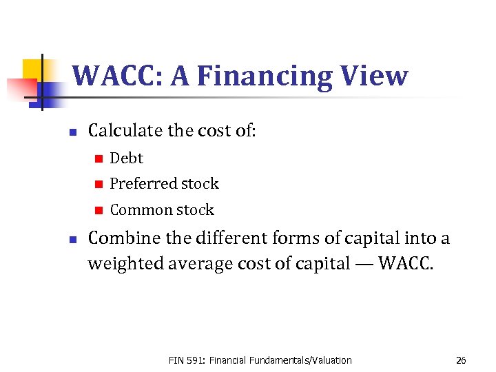WACC: A Financing View n Calculate the cost of: n n Preferred stock n n Debt Common stock Combine the different forms of capital into a weighted average cost of capital — WACC. FIN 591: Financial Fundamentals/Valuation 26

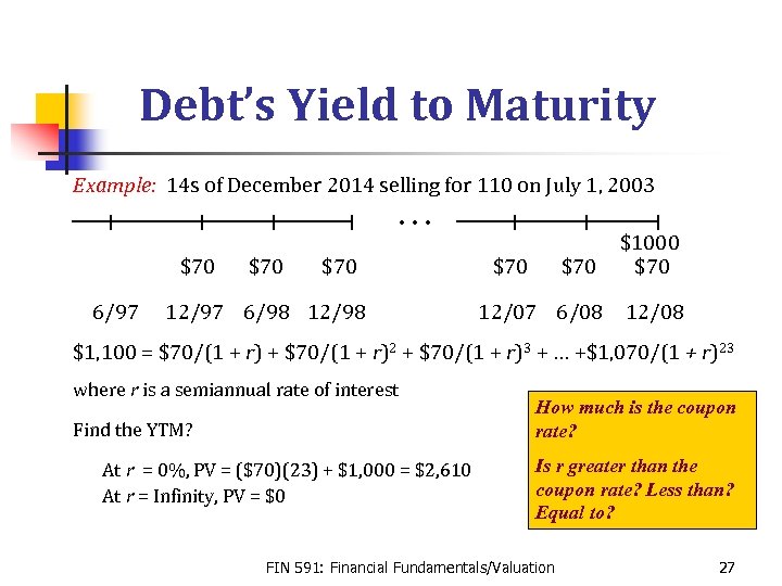Debt’s Yield to Maturity Example: 14 s of December 2014 selling for 110 on July 1, 2003 . . . $70 6/97 $70 12/97 6/98 12/98 $70 12/07 6/08 $1000 $70 12/08 $1, 100 = $70/(1 + r) + $70/(1 + r)2 + $70/(1 + r)3 + … +$1, 070/(1 + r)23 where r is a semiannual rate of interest Find the YTM? At r = 0%, PV = ($70)(23) + $1, 000 = $2, 610 At r = Infinity, PV = $0 How much is the coupon rate? Is r greater than the coupon rate? Less than? Equal to? FIN 591: Financial Fundamentals/Valuation 27

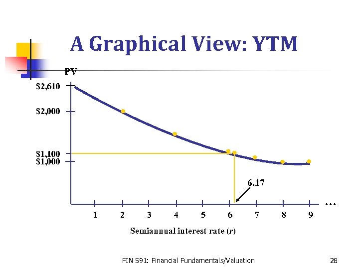A Graphical View: YTM PV $2, 610 $2, 000 $1, 100 $1, 000 6. 17 … 1 2 3 4 5 6 7 8 9 Semiannual interest rate (r) FIN 591: Financial Fundamentals/Valuation 28

Cost of Debt n Cost of debt to the firm is the YTM to investors adjusted for corporate taxes n Cost of debt = YTM * (1 - tc) n Example: A firm’s debt trades in the market to provide a YTM of 5%. If the firm’s tax rate is 34%, how much is the after-tax cost of debt? Answer: 5% * (1 -. 34) = 3. 30%. FIN 591: Financial Fundamentals/Valuation 29

Cost of Debt = YTM * (1 - tc) n Represents a good approximation if shareholders don’t default on debt service obligations n It is the rate shareholders promise the debt holders n Thus, bondholders’ expected return < YTM n See Exhibit 10. 1, page 211 of text. FIN 591: Financial Fundamentals/Valuation 30

Cost of Preferred Stock n n Preferred stock dividend is not tax deductible Cost is the market return earned by investors: Dividend / market price of preferred stock n Example: A preferred stock (par = $20) pays a $3 dividend annually. It currently trades in the market for $24. How much is the cost of the stock from the firm’s perspective? Answer: $3 / $24 = 12. 5%. FIN 591: Financial Fundamentals/Valuation 31

Cost of Equity n n Cost of equity is more difficult to calculate than either the cost of debt or the cost of preferred stock Methods commonly used: n M&M model n Dividend growth model (Gordon model) n Inverted price-earnings ratio n Security market line n Build-up approach. FIN 591: Financial Fundamentals/Valuation 32

Using Historic Returns n Estimating cost of capital using past returns is justified by “rational expectations” theory Investors’ expectations for returns that compensate them for risk can’t be systematically off target n The average of past returns is the return that investors expect to receive n Sometimes the return is higher; other times lower n However, errors are not systematic. n FIN 591: Financial Fundamentals/Valuation 33

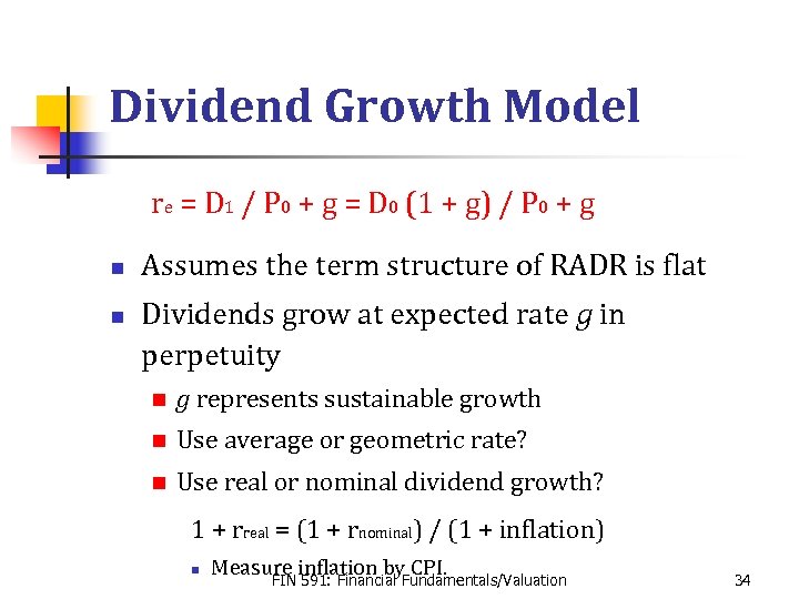Dividend Growth Model re = D 1 / P 0 + g = D 0 (1 + g) / P 0 + g n n Assumes the term structure of RADR is flat Dividends grow at expected rate g in perpetuity n g represents sustainable growth n Use average or geometric rate? n Use real or nominal dividend growth? 1 + rreal = (1 + rnominal) / (1 + inflation) n Measure inflation by CPI. FIN 591: Financial Fundamentals/Valuation 34

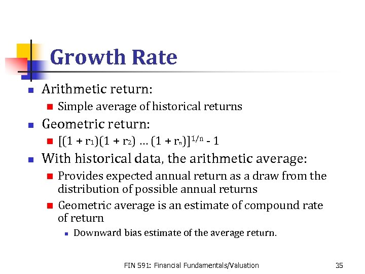Growth Rate n Arithmetic return: n n Geometric return: n n Simple average of historical returns [(1 + r 1)(1 + r 2) … (1 + rn)]1/n - 1 With historical data, the arithmetic average: Provides expected annual return as a draw from the distribution of possible annual returns n Geometric average is an estimate of compound rate of return n n Downward bias estimate of the average return. FIN 591: Financial Fundamentals/Valuation 35

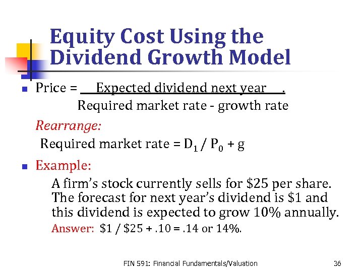Equity Cost Using the Dividend Growth Model n n Price = Expected dividend next year. Required market rate - growth rate Rearrange: Required market rate = D 1 / P 0 + g Example: A firm’s stock currently sells for $25 per share. The forecast for next year’s dividend is $1 and this dividend is expected to grow 10% annually. Answer: $1 / $25 +. 10 =. 14 or 14%. FIN 591: Financial Fundamentals/Valuation 36

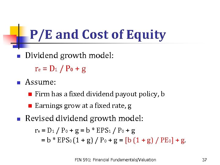P/E and Cost of Equity n Dividend growth model: re = D 1 / P 0 + g n Assume: n n n Firm has a fixed dividend payout policy, b Earnings grow at a fixed rate, g Revised dividend growth model: re = D 1 / P 0 + g = b * EPS 0 (1 + g) / P 0 + g = [b (1 + g) / PE 0] + g. FIN 591: Financial Fundamentals/Valuation 37

Problem with Dividend Model n n n Says nothing about risk! Returns should be based on perceived risk But not total risk n Investors able to diversify away some risk n Market only compensates for non- diversifiable or systematic risk. FIN 591: Financial Fundamentals/Valuation 38

The End FIN 591: Financial Fundamentals/Valuation 39