Lecture 3 The Aggregate Demand & Aggregate Supply

Lecture 3 The Aggregate Demand & Aggregate Supply

Lecture 3: The Aggregate Demand & Aggregate Supply 1. Aggregate Demand. 2. Aggregate Supply. 3. The Aggregate Demand-Aggregate Supply Model.

Lecture 3: The Aggregate Demand & Aggregate Supply Inventory – запаси Overheating – перегрів (економіки)

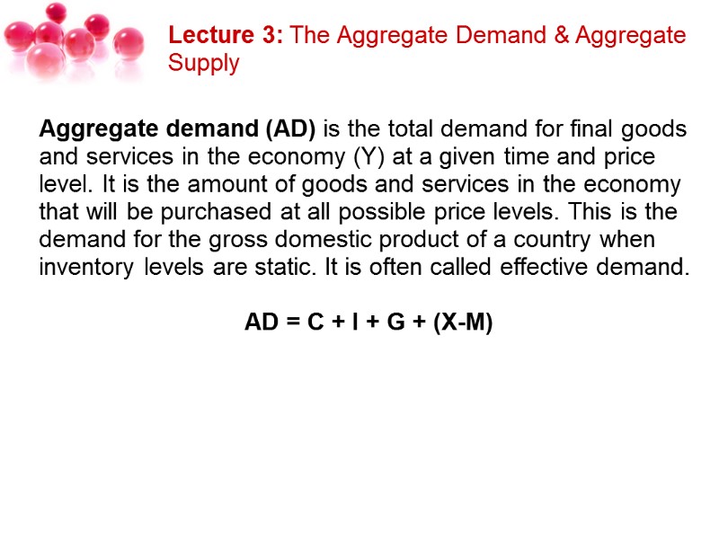
Lecture 3: The Aggregate Demand & Aggregate Supply Aggregate demand (AD) is the total demand for final goods and services in the economy (Y) at a given time and price level. It is the amount of goods and services in the economy that will be purchased at all possible price levels. This is the demand for the gross domestic product of a country when inventory levels are static. It is often called effective demand. AD = C + I + G + (X-M)

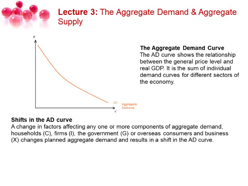
Lecture 3: The Aggregate Demand & Aggregate Supply The Aggregate Demand Curve The AD curve shows the relationship between the general price level and real GDP. It is the sum of individual demand curves for different sectors of the economy. Shifts in the AD curve A change in factors affecting any one or more components of aggregate demand, households (C), firms (I), the government (G) or overseas consumers and business (X) changes planned aggregate demand and results in a shift in the AD curve.

Lecture 3: The Aggregate Demand & Aggregate Supply Factors causing a shift in AD: Changes in Expectations. Current spending is affected by anticipated future income, profit, and inflation. Changes in Monetary Policy – i.e. a change in interest rates. Lower interest rates encourage firms to borrow and invest. Changes in Fiscal Policy. Fiscal Policy refers to changes in government spending, welfare benefits and taxation, and the amount that the government borrows. Economic events in the international economy. International factors such as the exchange rate and foreign income (e.g. the economic cycle in other countries.) Changes in household wealth. Wealth refers to the value of assets owned by consumers e.g. houses and shares.

Lecture 3: The Aggregate Demand & Aggregate Supply Aggregate supply is the total supply of goods and services that firms in a national economy plan on selling during a specific time period. It is the total amount of goods and services that firms are willing to sell at a given price level in an economy. Aggregate supply is determined by the supply side performance of the economy. It reflects the productive capacity of the economy and the costs of production in each sector.

Lecture 3: The Aggregate Demand & Aggregate Supply There are generally three forms of aggregate supply (AS). They are: 1. Short run aggregate supply (SRAS) - Within the time frame during which firms can change the amount of labor used but not capital (such as building new factories). This form demonstrates what happens to the economy when resources are underused. Upward shifts in SRAS generally increase output (Y) but don't increase price (P). The SRAS curve is nearly perfectly horizontal. It also calls Keynesian sector. The concept is that wages (price of labor) don't change over the short run.

Lecture 3: The Aggregate Demand & Aggregate Supply 2. Long run aggregate supply (LRAS) - Over the long run, only capital, labor, and technology affect the LRAS in the macroeconomic model because at this point everything in the economy is used optimally. In most situations, the LRAS is viewed as static because it shifts the slowest of the three. The LRAS is shown as perfectly vertical, reflecting economists belief that changes in aggregate demand (AD) have an only temporary change on the economy's total output. It is a Classical sector. 3. Medium run aggregate supply (MRAS) - As an interim between SRAS and LRAS, the MRAS form slopes upward and reflects when capital as well as labor can change. The MRAS curve is affected by capital, labor, technology, and wage rate. This sector calls Intermediate.

Lecture 3: The Aggregate Demand & Aggregate Supply Shifts in the AS curve can be caused by the following factors: Changes in size & quality of the labour force available for production. Changes in size & quality of capital stock through investment. Technological progress and the impact of innovation. Changes in factor productivity of both labour and capital. Changes in unit wage costs (wage costs per unit of output.) Changes in producer taxes and subsidies. Changes in inflation expectations - a rise in inflation expectations is likely to boost wage levels and cause AS to shift inwards.

Lecture 3: The Aggregate Demand & Aggregate Supply The AD-AS or Aggregate Demand-Aggregate Supply model is a macroeconomic model that explains price level and output through the relationship of aggregate demand and aggregate supply. It was first put forth by John Maynard Keynes in his work The General Theory of Employment, Interest, and Money. The AD-AS model is used to illustrate the Keynesian model of the business cycle. Movements of the two curves can be used to predict the effects that various exogenous events will have on two variables: real GDP and the price level.

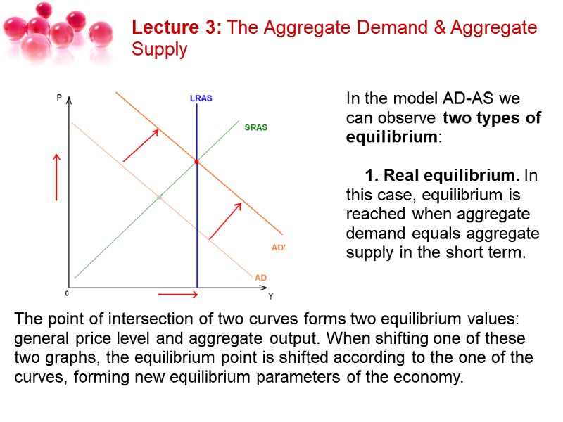
Lecture 3: The Aggregate Demand & Aggregate Supply In the model AD-AS we can observe two types of equilibrium: 1. Real equilibrium. In this case, equilibrium is reached when aggregate demand equals aggregate supply in the short term. The point of intersection of two curves forms two equilibrium values: general price level and aggregate output. When shifting one of these two graphs, the equilibrium point is shifted according to the one of the curves, forming new equilibrium parameters of the economy.

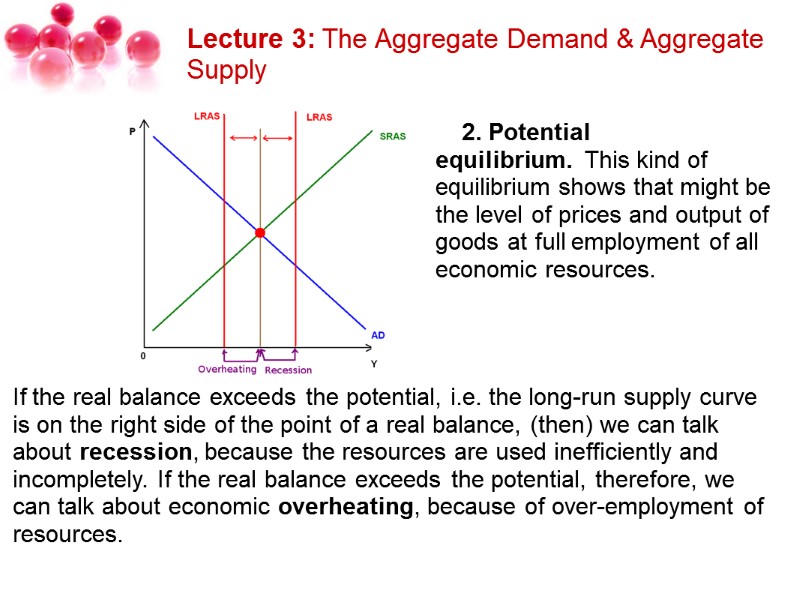
Lecture 3: The Aggregate Demand & Aggregate Supply 2. Potential equilibrium. This kind of equilibrium shows that might be the level of prices and output of goods at full employment of all economic resources. If the real balance exceeds the potential, i.e. the long-run supply curve is on the right side of the point of a real balance, (then) we can talk about recession, because the resources are used inefficiently and incompletely. If the real balance exceeds the potential, therefore, we can talk about economic overheating, because of over-employment of resources.

Fin