International Trade : Theory and Policy Lecture 5

International Trade : Theory and Policy Lecture 5 September, 2016 Instructor: Natalia Davidson Lecture is prepared by Prof. Sergey Kadochnikov, Natalia Davidson

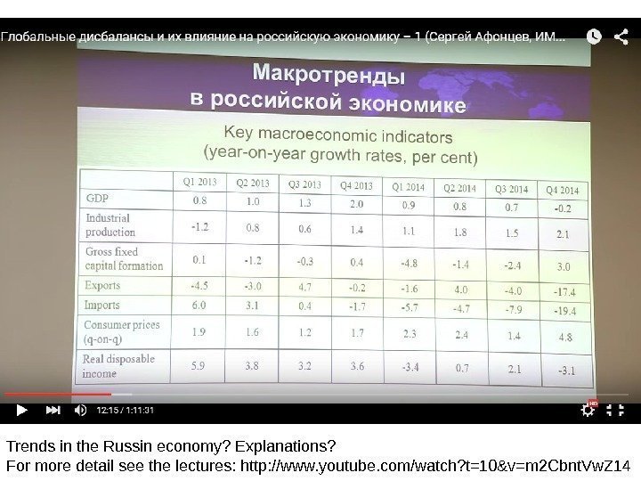
Trends in the Russin economy ? Explanations? For more detail see the lectures: http: //www. youtube. com/watch? t=10&v=m 2 Cbnt. Vw. Z

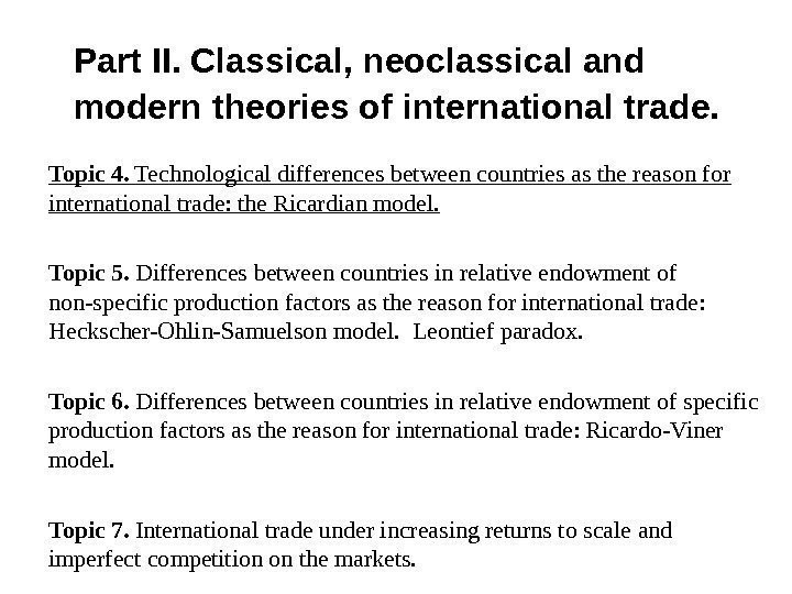
Part II. Classical, neoclassical and modern theories of international trade. Topic 4. Technological differences between countries as the reason for international trade: the Ricardian model. Topic 5. Differences between countries in relative endowment of non-specific production factors as the reason for international trade: Heckscher-Ohlin-Samuelson model. Leontief paradox. Topic 6. Differences between countries in relative endowment of specific production factors as the reason for international trade: Ricardo-Viner model. Topic 7. International trade under increasing returns to scale and imperfect competition on the markets.

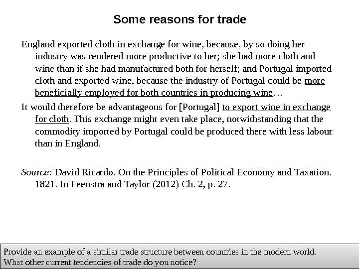
Some reasons for trade Engl and exported cloth in exchange for wine, because, by so doing her industry was rendered more productive to her; she had more cloth and wine than if she had manufactured both for herself; and Portugal imported cloth and exported wine, because the industry of Portugal could be more beneficially employed for both countries in producing wine … It would therefore be advantageous for [Portugal] to export wine in exchange for cloth. This exchange might even take place, notwithstanding that the commodity imported by Portugal could be produced there with less labour than in England. Source: David Ricardo. On the Principles of Political Economy and Taxation. 1821. In Feenstra and Taylor (2012) Ch. 2, p. 27. Provide an example of a similar trade structure between countries in the modern world. What other current tendencies of trade do you notice?

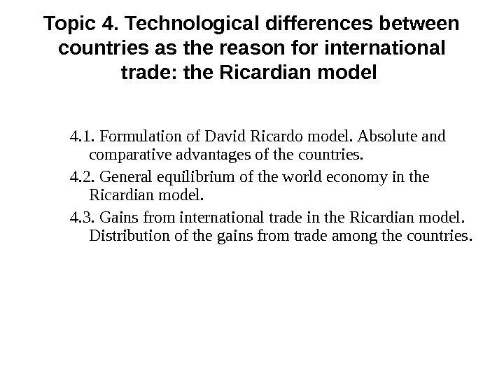
Topic 4. Technological differences between countries as the reason for international trade: the Ricardian model 4. 1. Formulation of David Ricardo model. Absolute and comparative advantages of the countries. 4. 2. General equilibrium of the world economy in the Ricardian model. 4. 3. Gains from international trade in the Ricardian model. Distribution of the gains from trade among the countries.

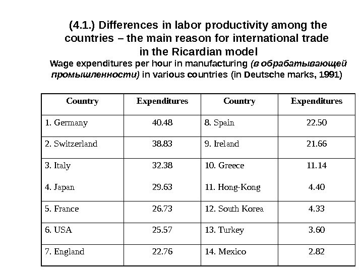
(4. 1. ) Differences in labor productivity among the countries – the main reason for international trade in the Ricardian model Wage expenditures per hour in manufacturing ( в обрабатывающей промышленности ) in various countries ( in Deutsche marks , 1991) Country Expenditures 1. Germany 40. 48 8. Spain 22. 50 2. Switzerland 38. 83 9. Ireland 21. 66 3. Italy 32. 38 10. Greece 11. 14 4. Japan 29. 63 11. Hong-Kong 4. 40 5. France 26. 73 12. South Korea 4. 33 6. USA 25. 57 13. Turkey 3. 60 7. England 22. 76 14. Mexico 2.

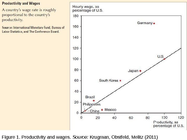
Figure 1. Productivity and wages. Source: Krugman, Obstfeld, Melitz (2011)

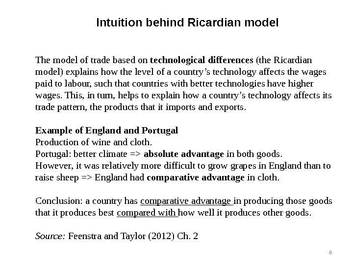
Intuition behind Ricardian model The model of trade based on technological differences (the Ricardian model) explains how the level of a country’s technology affects the wages paid to labour, such that countries with better technologies have higher wages. This, in turn, helps to explain how a country’s technology affects its trade pattern, the products that it imports and exports. Example of England Portugal Production of wine and cloth. Portugal: better climate => absolute advantage in both goods. However, it was relatively more difficult to grow grapes in England than to raise sheep => England had comparative advantage in cloth. Conclusion: a country has comparative advantage in producing those goods that it produces best compared with how well it produces other goods. Source: Feenstra and Taylor (2012) Ch.

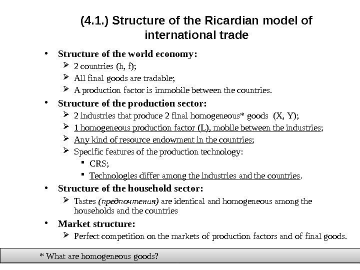
(4. 1. ) Structure of the Ricardian model of international trade • Structure of the world economy : 2 countries ( h, f); All final goods are tradable ; A production factor is immobile between the countries. • Structure of the production sector : 2 industries that produce 2 final homogeneous* goods ( X, Y); 1 homogeneous production factor ( L ), mobile between the industries ; Any kind of resource endowment in the countries ; Specific features of the production technology : CRS; Technologies differ among the industries and the countries. • Structure of the household sector : Tastes ( предпочтения ) are identical and homogeneous among the households and the countries • Market structure: Perfect competition on the markets of production factors and of final goods. * What are homogeneous goods?

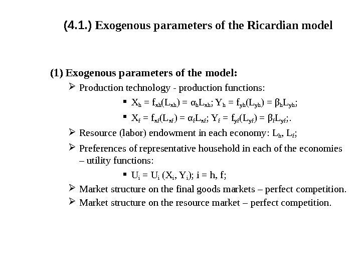
(4. 1. ) Exogenous parameters of the Ricardian model (1) Exogenous parameters of the model : Production technology — production functions : Х h = f xh (L xh ) = α h L xh ; Y h = f yh (L yh ) = β h L yh ; Х f = f xf (L xf ) = α f L xf ; Y f = f yf (L yf ) = β f L yf ; . Resource (labor) endowment in each economy : L h , L f ; Preferences of representative household in each of the economies – utility functions : U i = U i (X i , Y i ); i = h, f; Market structure on the final goods markets – perfect competition. Market structure on the resource market – perfect competition.

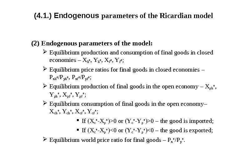
(4. 1. ) Endogenous parameters of the Ricardian model (2) Endogenous parameters of the model : Equilibrium production and consumption of final goods in closed economies – X h a , Y h a , X f a , Y f a ; Equilibrium price ratios for final goods in closed economies – P xh a / P yh a , P xf a / P yf a ; Equilibrium production of final goods in the open economy – X ph * , Y ph * , X pf * , Y pf * ; Equilibrium consumption of final goods in the open economy – X с h * , Y с h * , X с f * , Y с f * ; If ( X c * — X p * ) > 0 or ( Y c * — Y p * ) > 0 – the good is imported ; If ( X c * — X p * ) < 0 or ( Y c * — Y p * ) < 0 – the good is exported ; Equilibrium world price ratio for final goods – P x * / P y *.

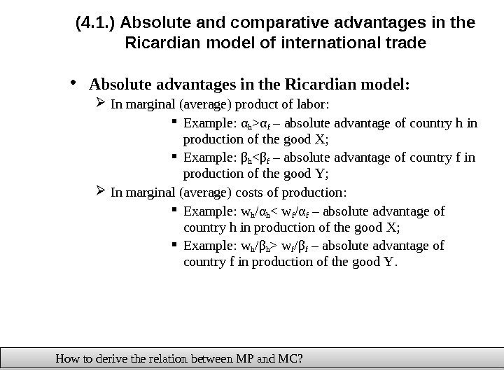
(4. 1. ) Absolute and comparative advantages in the Ricardian model of international trade • Absolute advantages in the Ricardian model : In marginal ( average ) product of labor : Example : α h > α f – absolute advantage of country h in production of the good Х; Example : β h < β f – absolute advantage of country f in production of the good Y ; In marginal ( average ) costs of production : Example : w h / α h w f / β f – absolute advantage of country f in production of the good Y. How to derive the relation between MP and MC?

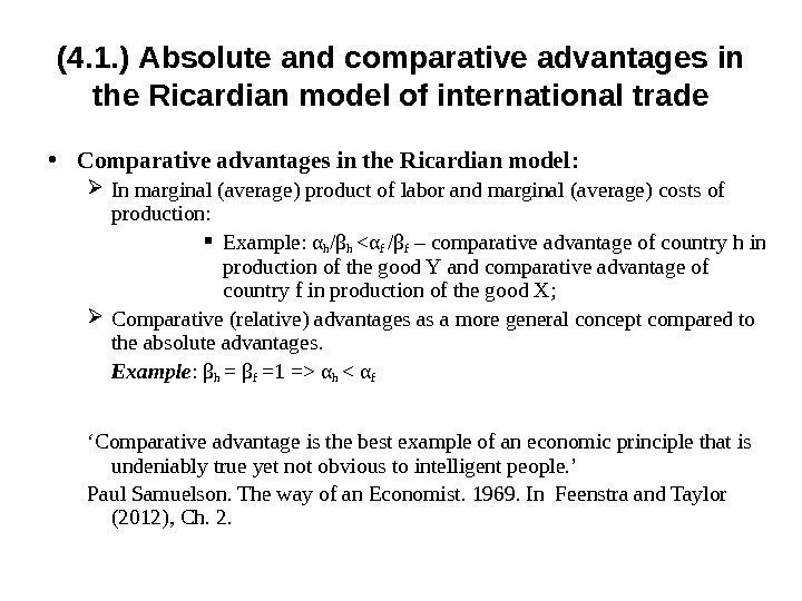
(4. 1. ) Absolute and comparative advantages in the Ricardian model of international trade • Comparative advantages in the Ricardian model : In marginal ( average ) product of labor and marginal ( average ) costs of production : Example : α h / β h α h < α f ‘ Comparative advantage is the best example of an economic principle that is undeniably true yet not obvious to intelligent people. ’ Paul Samuelson. The way of an Economist. 1969. In Feenstra and Taylor (2012), Ch. 2.

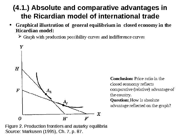
(4. 1. ) Absolute and comparative advantages in the Ricardian model of international trade • Graphical illustration of general equilibrium in closed economy in the Ricardian model : Graph with production possibility curves and indifference curves Figure 2. Production frontiers and autarky equilibria Source: Markusen (1995), Ch. 7, p. 87. Conclusion : Price ratio in the closed economy reflects comparative (relative) advantage of the country. Question: How is absolute advantage reflected on the graph?

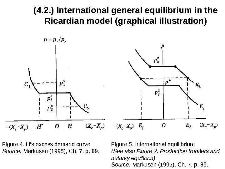
(4. 2. ) International general equilibrium in the Ricardian model ( graphical illustration ) • Derivation of the excess demand function in the Ricardian model : Specific features of the excess demand curve as reflection of production sector characteristics in the Ricardian model • International general equilibrium in the Ricardian model – defining the equilibrium prices ( graphical illustration ): Using excess demand curves ; Using production possibility curves and indifference curves.

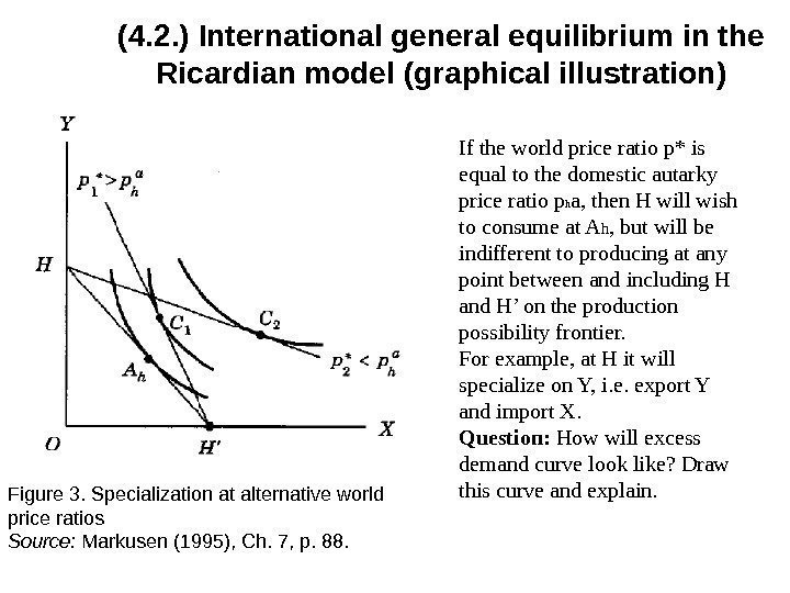
(4. 2. ) International general equilibrium in the Ricardian model ( graphical illustration ) Figure 3. Specialization at alternative world price ratios Source: Markusen (1995), Ch. 7, p. 88. If the world price ratio p* is equal to the domestic autarky price ratio p h a, then H will wish to consume at A h , but will be indifferent to producing at any point between and including H and H’ on the production possibility frontier. For example, at H it will specialize on Y, i. e. export Y and import X. Question: How will excess demand curve look like? Draw this curve and explain.

(4. 2. ) International general equilibrium in the Ricardian model ( graphical illustration ) Figure 4. H’s excess demand curve Source: Markusen (1995), Ch. 7, p. 89. Figure 5. International equilibrium (See also Figure 2. Production frontiers and autarky equilibria) Source: Markusen (1995), Ch. 7, p. 89.

Question: based on Figure 2. Production frontiers and autarky equilibria , draw the world price, indifference curves in open economy; show production points in open economy, export and import of the countries, and gains from trade of each country (in terms of utility). (4. 2. ) International general equilibrium in the Ricardian model ( graphical illustration )

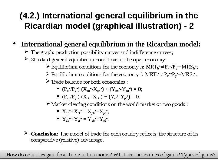
(4. 2. ) International general equilibrium in the Ricardian model ( graphical illustration ) — 2 • International general equilibrium in the Ricardian model: The graph: production possibility curves and indifference curves ; Standard general equilibrium conditions in the open economy : Equilibrium conditions for the economy h : MRTh* Px* / Py* = MRSh* ; Equilibrium conditions for the economy f : MRT f* Px* / Py* = MRSf* ; Trade balance for both economies : ( P x* / Py* ) ( Xch* — Xph* ) + ( Ych* — Yph* ) = 0; ( P x* / Py* ) ( Xcf* — Xpf* ) + ( Ycf* — Ypf* ) = 0. Market clearing conditions on the world market of two goods : X ch* + Xсf* = Xph* +Xpf* ; Y ch* + Yсf* = Yph* +Ypf*. Conclusion : The model of trade for each country reflects the structure of its comparative (relative) advantage. How do countries gain from trade in this model? What are the sources of gains? Types of gains?

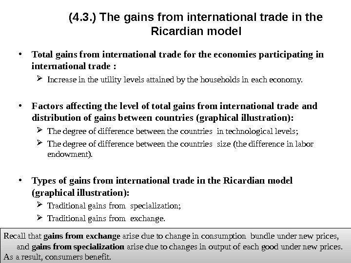
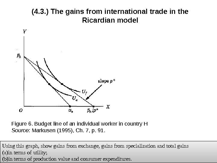
(4. 3. ) The gains from international trade in the Ricardian model • Total gains from international trade for the economies participating in international trade : Increase in the utility levels attained by the households in each economy. • Factors affecting the level of total gains from international trade and distribution of gains between countries ( graphical illustration ): The degree of difference between the countries in technological levels ; The degree of difference between the countries size ( the difference in labor endowment ). • Types of gains from international trade in the Ricardian model ( graphical illustration ): Traditional gains from specialization; Traditional gains from exchange. Recall that gains from exchange arise due to change in consumption bundle under new prices, and gains from specialization arise due to changes in output of each good under new prices. As a result, consumers benefit.

(4. 3. ) The gains from international trade in the Ricardian model Figure 6. Budget line of an individual worker in country H Source: Markusen (1995), Ch. 7, p. 91. Using this graph, show gains from exchange, gains from specialization and total gains (a) in terms of utility; (b) in terms of production value and consumer expenditures.

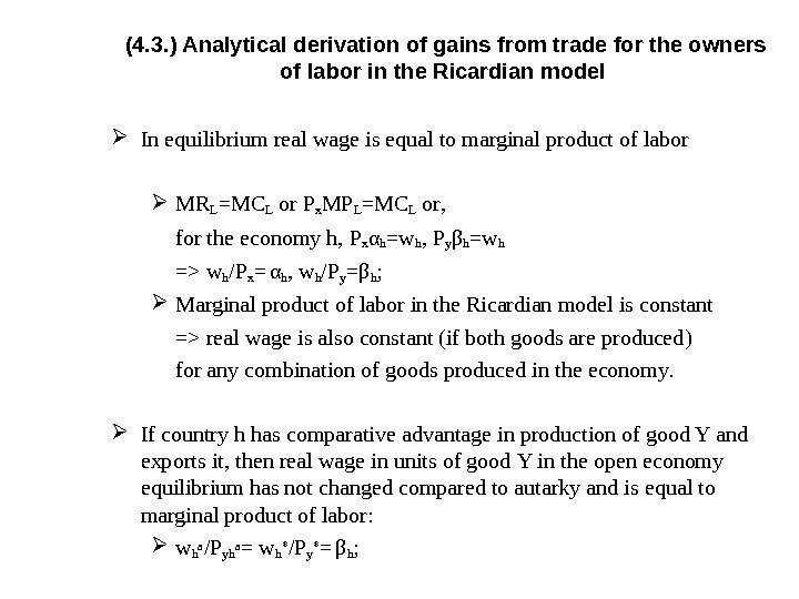
(4. 3. ) Analytical derivation of gains from trade for the owners of labor in the Ricardian model In equilibrium real wage is equal to marginal product of labor MR L =MC L or P x MP L =MC L or , for the economy h, P x α h = w h , P y β h = w h => w h / P x = α h , w h / P y = β h ; Marginal product of labor in the Ricardian model is constant => real wage is also constant (if both goods are produced) for any combination of goods produced in the economy. If country h has comparative advantage in production of good Y and exports it , then real wage in units of good Y in the open economy equilibrium has not changed compared to autarky and is equal to marginal product of labor : w h а / P yh а = w h * / P y * = β h ;

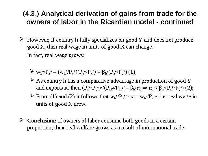
(4. 3. ) Analytical derivation of gains from trade for the owners of labor in the Ricardian model — continued However, if country h fully specializes on good Y and does not produce good X, then real wage in units of good X can change. In fact, real wage grows: w h * / P x * = (w h * / P y * )(P y * / P x * ) = β h /(P x * / P y * ) (1) ; As country h has a comparative advantage in production of good Y and exports it , then (P x * / P y * ) < (P xh а / P yh а ) = β h / α h α h = w h а / P xh а ; i. e. real wage in units of good X grew. Conclusion : If owners of labor consume both goods in a certain proportion, their real welfare grows as a result of international trade.

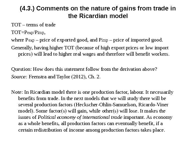
TOT – terms of trade TOT=P exp /P imp , where P exp – price of exported good, and P imp – price of imported good. Generally, having higher TOT (because of high export prices or low import prices) will lead to higher real wages and therefore will benefit workers. Question: How does this statement follow from the derivation above? Source: Feenstra and Taylor (2012), Ch. 2. Note: In Ricardian model there is one production factor, labour. It necessarily benefits from trade. In the next models that we will study there will be several production factors (Heckscher-Ohlin-Samuelson, Ricardo-Viner model). Some factor(s) will gain, while other(s) will lose. It makes the issues of Political economy of international trade important. As economy as a whole benefits, all production factors can eventually benefit, if a certain redistribution of income among production factors takes place. (4. 3. ) Comments on the nature of gains from trade in the Ricardian model

(1) Exercise sessions 3, 4 (2) Think about topics for reports during exercise sessions; work on a paper review ( due 1 November 2016 ) and presentation Office hours: Friday 13: 50 – 14: 30, room 216. E-mail: natalya. davidson@gmail. com (Наталья Борисовна Давидсон)Homework

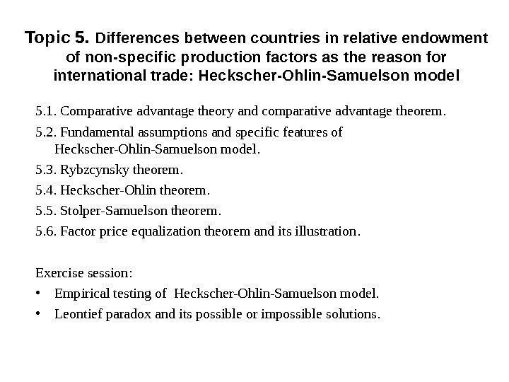
Topic 5. Differences between countries in relative endowment of non-specific production factors as the reason for international trade: Heckscher-Ohlin-Samuelson model 5. 1. Comparative advantage theory and comparative advantage theorem. 5. 2. Fundamental assumptions and specific features of Heckscher-Ohlin-Samuelson model. 5. 3. Rybzcynsky theorem. 5. 4. Heckscher-Ohlin theorem. 5. 5. Stolper-Samuelson theorem. 5. 6. Factor price equalization theorem and its illustration. Exercise session: • Empirical testing of Heckscher-Ohlin-Samuelson model. • Leontief paradox and its possible or impossible solutions.