Each function has a specific order called

Each function has a specific order, called syntax, which must be strictly followed for the function to work correctly. Syntax Order: All functions begin with the = sign. After the = sign define the function name (e. g. , Sum). Then there will be an argument. An argument is the cell range or cell references that are enclosed by parentheses. If there is more than one argument, separate each by a comma.

An example of a function with one argument that adds a range of cells, A 3 through A 9: An example of a function with more than one argument that calculates the sum of two cell ranges:

There are many different functions in Excel 2007. Some of the more common functions include:

SUM - summation adds a range of cells together. AVERAGE - average calculates the average of a range of cells. COUNT - counts the number of chosen data in a range of cells. MAX - identifies the largest number in a range of cells. MIN - identifies the smallest number in a range of cells.

Interest Rates Loan Payments Depreciation Amounts

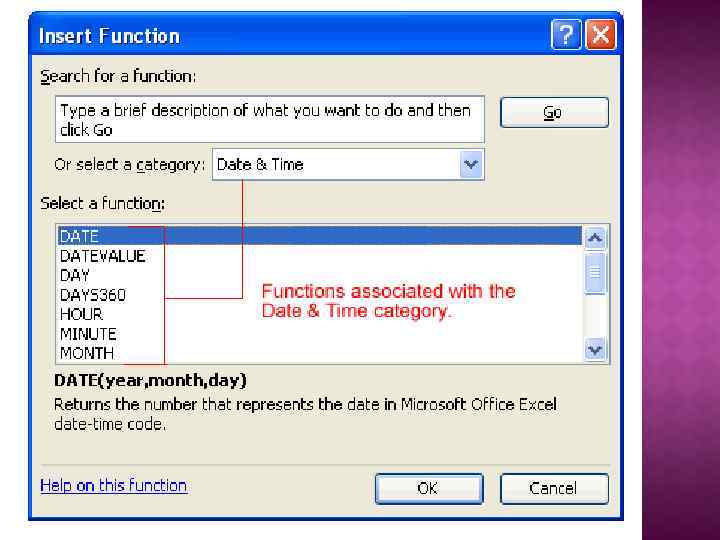
DATE - Converts a serial number to a day of the month Day of Week DAYS 360 - Calculates the number of days between two dates based on a 360 -day year TIME - Returns the serial number of a particular time HOUR - Converts a serial number to an hour MINUTE - Converts a serial number to a minute TODAY - Returns the serial number of today's date MONTH - Converts a serial number to a month YEAR - Converts a serial number to a year

Select the Formulas tab. Locate the Function Library group. From here, you can access all the available functions. Select the cell where you want the function to appear. In this example, select G 42. Select the drop-down arrow next to the Auto. Sum command. Select Sum. A formula will appear in the selected cell, G 42.

Press the Enter key or Enter button on the formula bar. The total will appear.

To Edit a Function: Select the cell where the function is defined. Insert the cursor in the formula bar. Edit the range by deleting and changing necessary cell numbers.

To Calculate the Sum of Two Arguments: Select the cell where you want the function to appear. In this example, G 44. Click the Insert Function command on the Formulas tab. A dialog box appears. SUM is selected by default. Click OK and the Function Arguments dialog box appears so that you can enter the range of cells for the function.

Insert the cursor in the Number 1 field. In the spreadsheet, select the first range of cells. In this example, G 21 through G 26. The argument appears in the Number 1 field. Insert the cursor in the Number 2 field. In the spreadsheet, select the second range of cells. In this example, G 40 through G 41. The argument appears in the Number 2 field.

Select the cell where you want the function to appear. Click the drop-down arrow next to the Auto. Sum command. Select Average. Click on the first cell (in this example, C 8) to be included in the formula. Left-click and drag the mouse to define a cell range (C 8 through cell C 20, in this example). Click the Enter icon to calculate the average.

To Access Other Functions in Excel: Using the point-click-drag method, select a cell range to be included in the formula. On the Formulas tab, click on the drop-down part of the Auto. Sum button. If you don't see the function you want to use (Sum, Average, Count, Max, Min), display additional functions by selecting More Functions. The Insert Function dialog box opens. There are three ways to locate a function in the Insert Function dialog box: You can type a question in the Search for a function box and click GO, or You can scroll through the alphabetical list of functions in the Select a function field, or You can select a function category in the Select a category drop-down list and review the corresponding function names in the Select a function field.

A Microsoft Excel spreadsheet can contain a great deal of information. With more rows and columns than previous versions, Excel 2007 gives you the ability to analyze and work with an enormous amount of data. To most effectively use this data, you may need to manipulate this data in different ways. Sorting lists is a common spreadsheet task that allows you to easily reorder your data. The most common type of sorting is alphabetical ordering, which you can do in ascending or descending order.

Select a cell in the column you want to sort (In this example, we choose a cell in column A). Click the Sort & Filter command in the Editing group on the Home tab. Select Sort A to Z. Now the information in the Category column is organized in alphabetical order. You can Sort in reverse alphabetical order by choosing Sort Z to A in the list.

Select a cell in the column you want to sort (a column with numbers). Click the Sort & Filter command in the Editing group on the Home tab. Select From Smallest to Largest. Now the information is organized from the smallest to largest amount.

Click the Sort & Filter command in the Editing group on the Home tab. Select Custom Sort from the list to open the dialog box. OR Select the Data tab. Locate the Sort and Filter group. Click the Sort command to open the Custom Sort dialog box. From here, you can sort by one item, or multiple items.

The spreadsheet has been sorted. All the categories are organized in alphabetical order, and within each category, the unit cost is arranged from smallest to largest. Remember all of the information and data is still here. It's just in a different order.

Filtering, or temporarily hiding, data in a spreadsheet very easy. This allows you to focus on specific spreadsheet entries. To Filter Data: Click the Filter command on the Data tab. Drop-down arrows will appear beside each column heading. Click the drop-down arrow next to the heading you would like to filter. For example, if you would like to only view data regarding Flavors, click the drop-down arrow next to Category.

Uncheck Select All. Choose Flavor. Click OK. All other data will be filtered, or hidden, and only the Flavor data is visible. To Clear One Filter: Select one of the drop-down arrows next to a filtered column. Choose Clear Filter From. To remove all filters, click the Filter command.

A chart is a tool you can use in Excel to communicate your data graphically. Charts allow your audience to more easily see the meaning behind the numbers in the spreadsheet, and make showing comparisons and trends a lot easier. Creating a Charts can be a useful way to communicate data. When you insert a chart in Excel, it appears in the selected worksheet with the source data, by default.