Chapter Six Demand Properties of Demand Functions

Chapter Six Demand

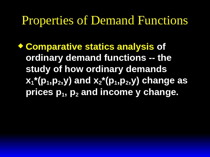
Properties of Demand Functions Comparative statics analysis of ordinary demand functions — the study of how ordinary demands x 1 *(p 1 , p 2 , y) and x 2 *(p 1 , p 2 , y) change as prices p 1 , p 2 and income y change.

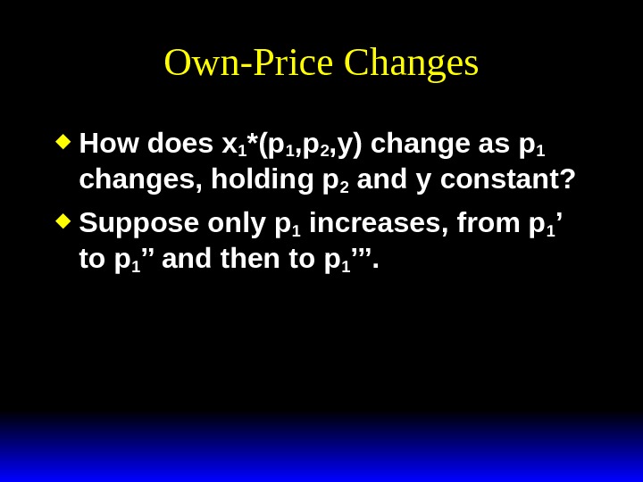
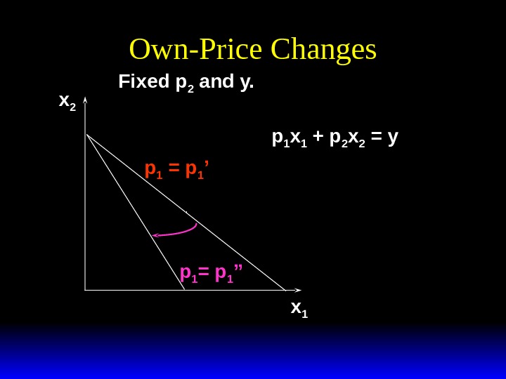
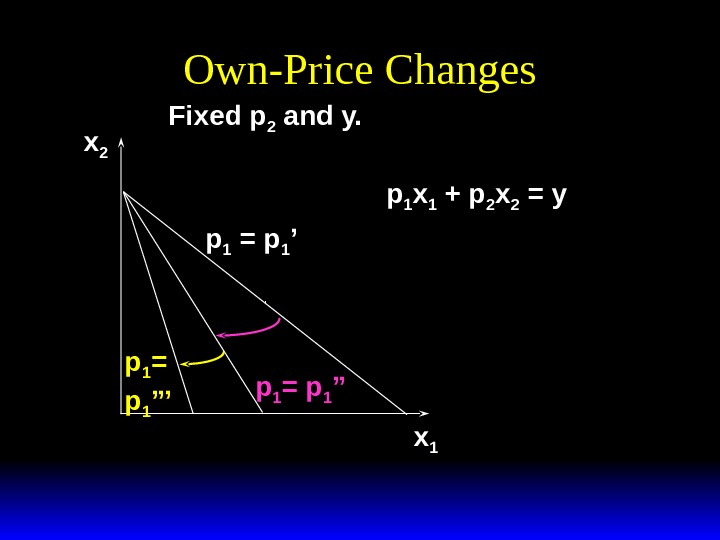
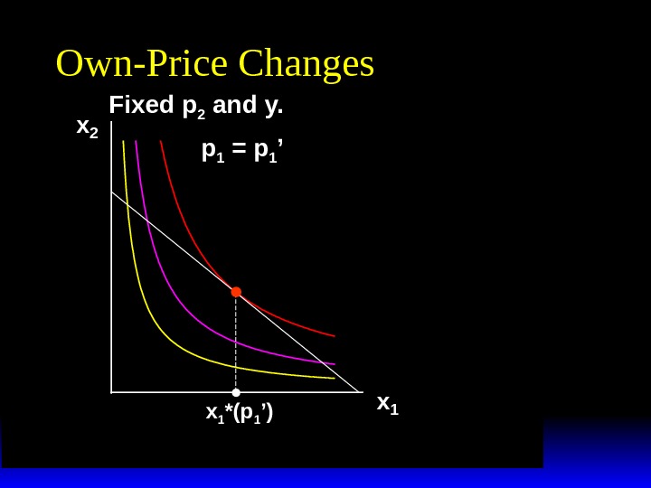
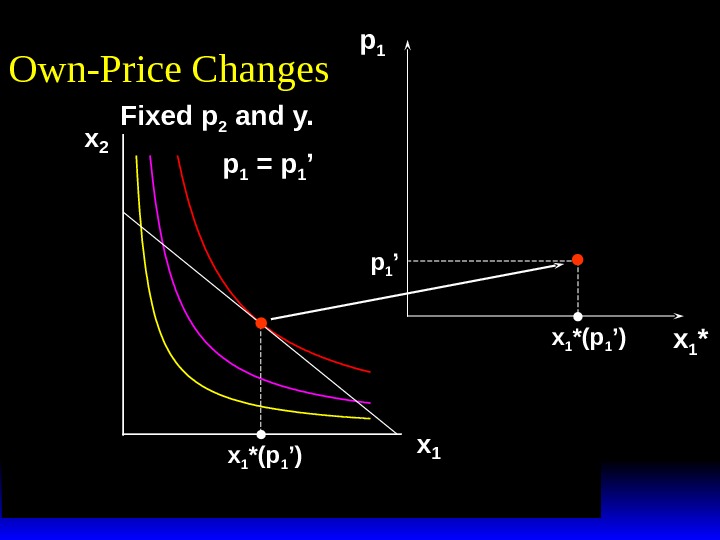
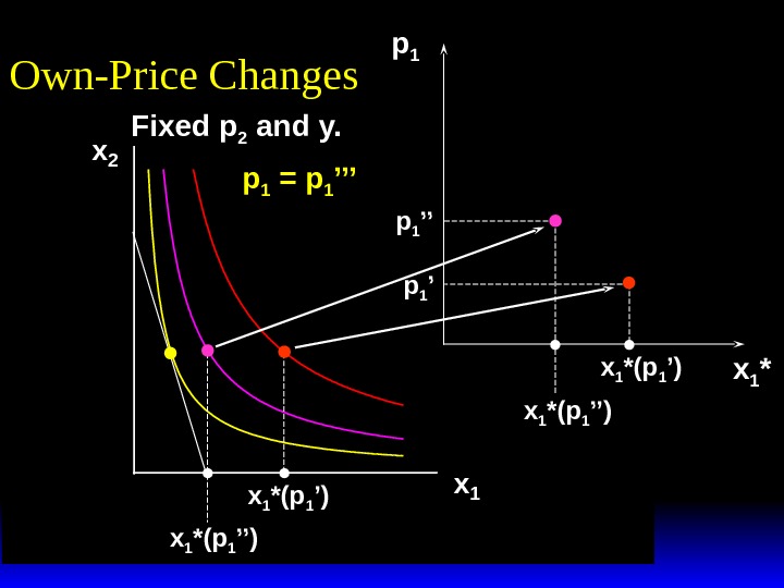
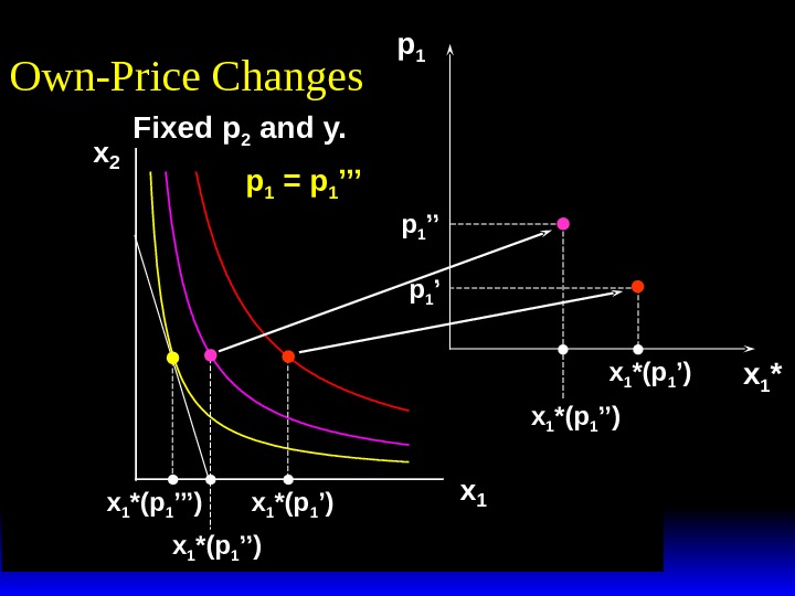
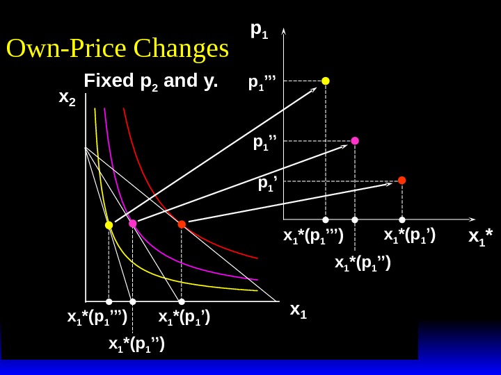
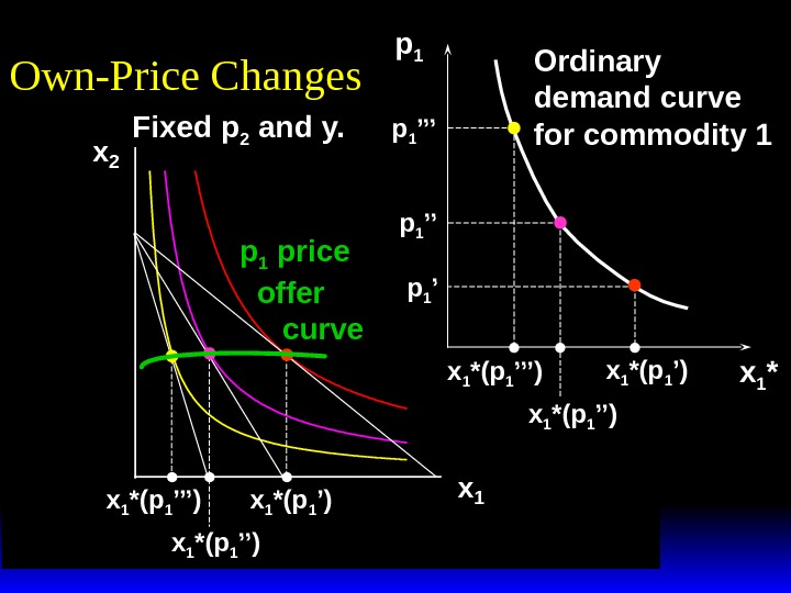
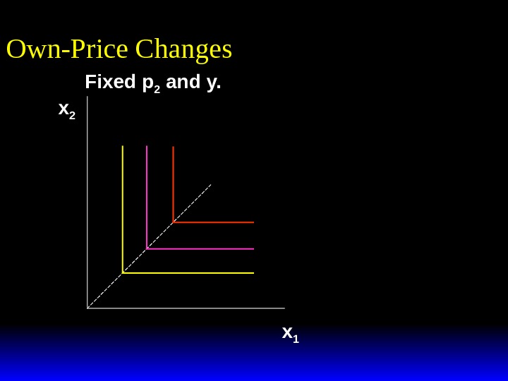
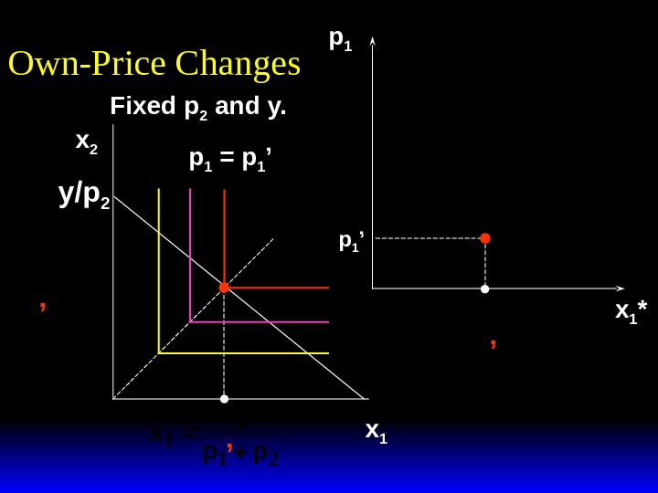
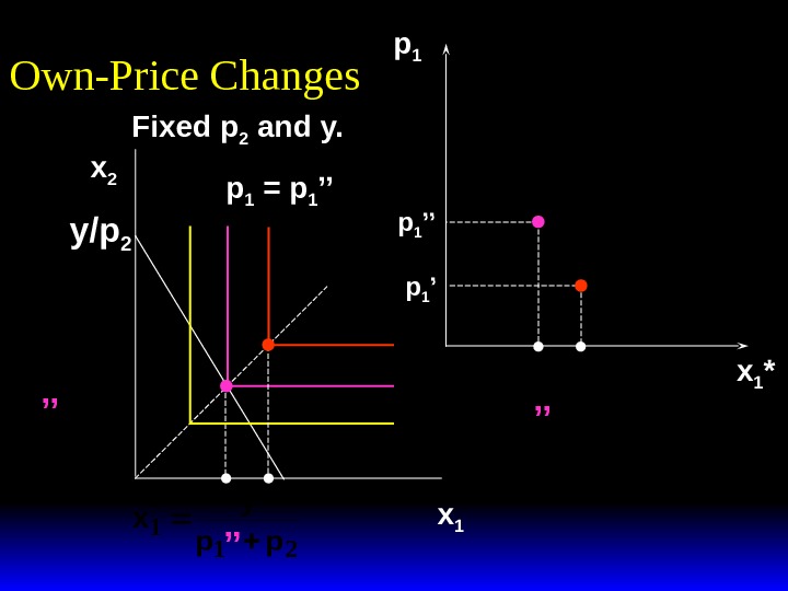
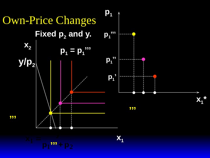
Own-Price Changes How does x 1 *(p 1 , p 2 , y) change as p 1 changes, holding p 2 and y constant? Suppose only p 1 increases, from p 1 ’ to p 1 ’’ and then to p 1 ’’’.

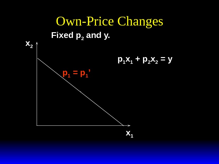
x 1 x 2 p 1 = p 1 ’Fixed p 2 and y. p 1 x 1 + p 2 x 2 = y. Own-Price Changes

Own-Price Changes x 1 x 2 p 1 = p 1 ’’p 1 = p 1 ’Fixed p 2 and y. p 1 x 1 + p 2 x 2 = y

Own-Price Changes x 1 x 2 p 1 = p 1 ’’’ Fixed p 2 and y. p 1 = p 1 ’ p 1 x 1 + p 2 x 2 = y

x 2 x 1 p 1 = p 1 ’Own-Price Changes Fixed p 2 and y.

x 2 x 1 *(p 1 ’)Own-Price Changes p 1 = p 1 ’Fixed p 2 and y.

x 2 x 1 *(p 1 ’) p 1 x 1 *(p 1 ’)p 1 ’ x 1 *Own-Price Changes Fixed p 2 and y. p 1 = p 1 ’

x 2 x 1 *(p 1 ’) p 1 x 1 *(p 1 ’)p 1 ’p 1 = p 1 ’’ x 1 *Own-Price Changes Fixed p 2 and y.

x 2 x 1 *(p 1 ’) x 1 *(p 1 ’’) p 1 x 1 *(p 1 ’)p 1 ’p 1 = p 1 ’’ x 1 *Own-Price Changes Fixed p 2 and y.

x 2 x 1 *(p 1 ’) x 1 *(p 1 ’’) p 1 x 1 *(p 1 ’) x 1 *(p 1 ’’)p 1 ’’ x 1 *Own-Price Changes Fixed p 2 and y.

x 2 x 1 *(p 1 ’) x 1 *(p 1 ’’) p 1 x 1 *(p 1 ’) x 1 *(p 1 ’’)p 1 ’’p 1 = p 1 ’’’ x 1 *Own-Price Changes Fixed p 2 and y.

x 2 x 1 *(p 1 ’’’) x 1 *(p 1 ’’) p 1 x 1 *(p 1 ’) x 1 *(p 1 ’’)p 1 ’’p 1 = p 1 ’’’ x 1 *Own-Price Changes Fixed p 2 and y.

x 2 x 1 *(p 1 ’’’) x 1 *(p 1 ’’) p 1 x 1 *(p 1 ’) x 1 *(p 1 ’’)p 1 ’’p 1 ’’’ x 1 *Own-Price Changes Fixed p 2 and y.

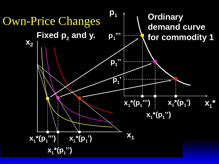
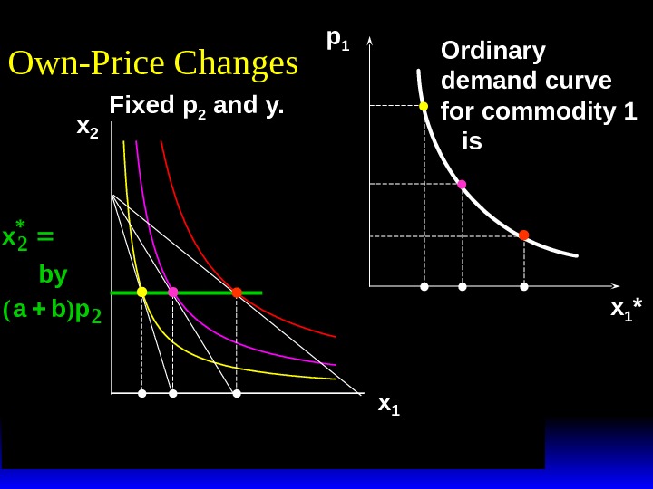
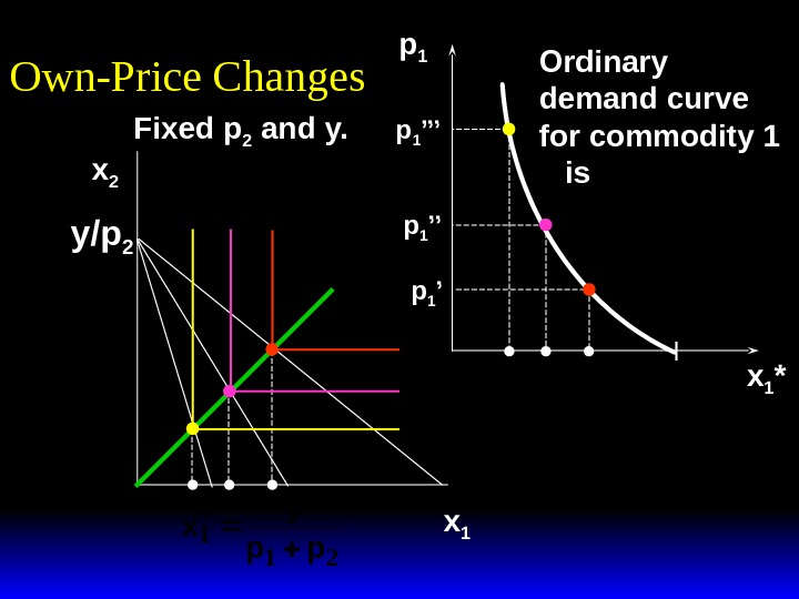
x 2 x 1 *(p 1 ’’’) x 1 *(p 1 ’’) p 1 x 1 *(p 1 ’) x 1 *(p 1 ’’)p 1 ’’p 1 ’’’ x 1 *Own-Price Changes Ordinary demand curve for commodity 1 Fixed p 2 and y.

x 2 x 1 *(p 1 ’’’) x 1 *(p 1 ’’) p 1 x 1 *(p 1 ’) x 1 *(p 1 ’’)p 1 ’’p 1 ’’’ x 1 *Own-Price Changes Ordinary demand curve for commodity 1 Fixed p 2 and y.

x 2 x 1 *(p 1 ’’’) x 1 *(p 1 ’’) p 1 x 1 *(p 1 ’) x 1 *(p 1 ’’)p 1 ’’p 1 ’’’ x 1 *Own-Price Changes Ordinary demand curve for commodity 1 price offer curve. Fixed p 2 and y.

Own-Price Changes The curve containing all the utility-maximizing bundles traced out as p 1 changes, with p 2 and y constant, is the p 1 — price offer curve. The plot of the x 1 -coordinate of the p 1 — price offer curve against p 1 is the ordinary demand curve for commodity 1.

Own-Price Changes What does a p 1 price-offer curve look like for Cobb-Douglas preferences?

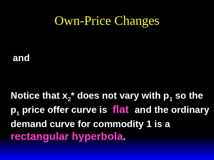
Own-Price Changes What does a p 1 price-offer curve look like for Cobb-Douglas preferences? Take Then the ordinary demand functions for commodities 1 and 2 are Uxxxx ab (, ).

Own-Price Changesxppy a ab y p 112 1 * (, , ) xppy b ab y p 212 2 * (, , ). and Notice that x 2 * does not vary with p 1 so the p 1 price offer curve is

Own-Price Changesxppy a ab y p 112 1 * (, , ) xppy b ab y p 212 2 * (, , ). and Notice that x 2 * does not vary with p 1 so the p 1 price offer curve is flat

Own-Price Changesxppy a ab y p 112 1 * (, , ) xppy b ab y p 212 2 * (, , ). and Notice that x 2 * does not vary with p 1 so the p 1 price offer curve is flat and the ordinary demand curve for commodity 1 is a

Own-Price Changesxppy a ab y p 112 1 * (, , ) xppy b ab y p 212 2 * (, , ). and Notice that x 2 * does not vary with p 1 so the p 1 price offer curve is flat and the ordinary demand curve for commodity 1 is a rectangular hyperbola.

x 1 *(p 1 ’’’) x 1 *(p 1 ’’)x 2 x 1 Own-Price Changes Fixed p 2 and y. x by abp 2 2 * () x ay abp 1 1 * ()

x 1 *(p 1 ’’’) x 1 *(p 1 ’’)x 2 x 1 p 1 x 1 *Own-Price Changes Ordinary demand curve for commodity 1 is. Fixed p 2 and y. x by abp 2 2 * () x ay abp 1 1 * ()

Own-Price Changes What does a p 1 price-offer curve look like for a perfect-complements utility function?

Own-Price Changes What does a p 1 price-offer curve look like for a perfect-complements utility function? Uxxxx(, )min, . 1212 Then the ordinary demand functions for commodities 1 and 2 are

Own-Price Changesxppy y pp 112212 12 ** (, , ).

Own-Price Changesxppy y pp 112212 12 ** (, , ). With p 2 and y fixed, higher p 1 causes smaller x 1 * and x 2 *.

Own-Price Changesxppy y pp 112212 12 ** (, , ). With p 2 and y fixed, higher p 1 causes smaller x 1 * and x 2 *. pxx y p 112 2 0, . ** As

Own-Price Changesxppy y pp 112212 12 ** (, , ). With p 2 and y fixed, higher p 1 causes smaller x 1 * and x 2 *. pxx y p 112 2 0, . ** As pxx 1120, . ** As

Fixed p 2 and y. Own-Price Changes x 1 x

p 1 x 1 *Fixed p 2 and y. x y pp 2 12 * x y pp 1 12 * Own-Price Changes x 1 x 2 p 1 ’ x y pp 1 12 * ’p 1 = p 1 ’ ’ ’y/p

p 1 x 1 *Fixed p 2 and y. x y p p 2 1 2* x y pp 1 12 * Own-Price Changes x 1 x 2 p 1 ’’p 1 = p 1 ’’ ’’ x y pp 1 12 * ’’ ’’y/p

p 1 x 1 *Fixed p 2 and y. x y pp 2 12 * x y pp 1 12 * Own-Price Changes x 1 x 2 p 1 ’’p 1 ’’’ x y pp 1 12 * p 1 = p 1 ’’’ ’’’y/p

p 1 x 1 *Ordinary demand curve for commodity 1 is. Fixed p 2 and y. x y pp 2 12 * x y pp 1 12 *. Own-Price Changes x 1 x 2 p 1 ’’p 1 ’’’ y p 2 y/p

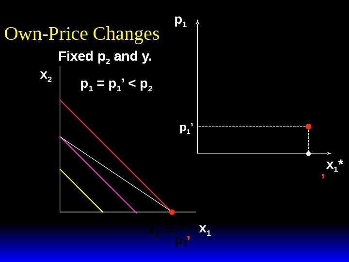
Own-Price Changes What does a p 1 price-offer curve look like for a perfect-substitutes utility function? Uxxxx(, ). 1212 Then the ordinary demand functions for commodities 1 and 2 are

Own-Price Changesxppy ifpp ypifpp 112 12 112 0 * (, , ) , /, xppy ifpp ypifpp 212 12 212 0 * (, , ) , /, . and

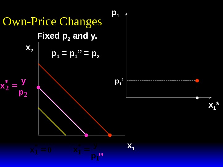
Fixed p 2 and y. Own-Price Changes x 2 x 1 Fixed p 2 and y. x 20 * x y p 1 1 * p 1 = p 1 ’ < p 2 ’

Fixed p 2 and y. Own-Price Changes x 2 x 1 p 1 x 1 *Fixed p 2 and y. x 20 * x y p 1 1 * p 1 ’p 1 = p 1 ’ < p 2 ’ x y p 1 1 * ’

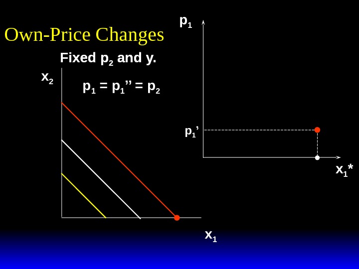
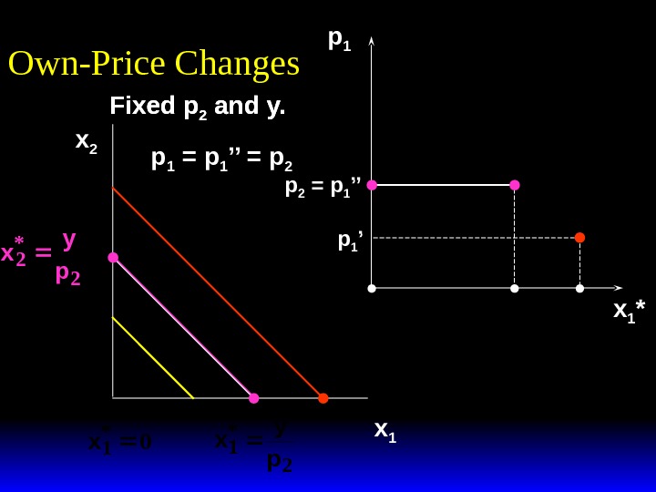
Fixed p 2 and y. Own-Price Changes x 2 x 1 p 1 x 1 *Fixed p 2 and y. p 1 ’p 1 = p 1 ’’ = p

Fixed p 2 and y. Own-Price Changes x 2 x 1 p 1 x 1 *Fixed p 2 and y. p 1 ’p 1 = p 1 ’’ = p

Fixed p 2 and y. Own-Price Changes x 2 x 1 p 1 x 1 *Fixed p 2 and y. x 20 * x y p 1 1 * p 1 ’p 1 = p 1 ’’ = p 2 ’’ x 10 * x y p 2 2 *

Fixed p 2 and y. Own-Price Changes x 2 x 1 p 1 x 1 *Fixed p 2 and y. x 20 * x y p 1 2 * p 1 ’p 1 = p 1 ’’ = p 2 x 10 * x y p 2 2 * 01 2 x y p * p 2 = p 1 ’’

Fixed p 2 and y. Own-Price Changes x 2 x 1 p 1 x 1 *Fixed p 2 and y. x y p 2 2 * x 10 * p 1 ’’’ x 10 * p 2 = p 1 ’’

Fixed p 2 and y. Own-Price Changes x 2 x 1 p 1 x 1 *Fixed p 2 and y. p 1 ’p 2 = p 1 ’’’x y p 1 1* 01 2 x y p * y p 2 p 1 price offer curve Ordinary demand curve for commodity

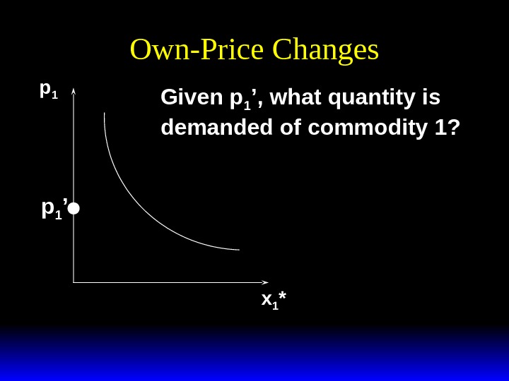
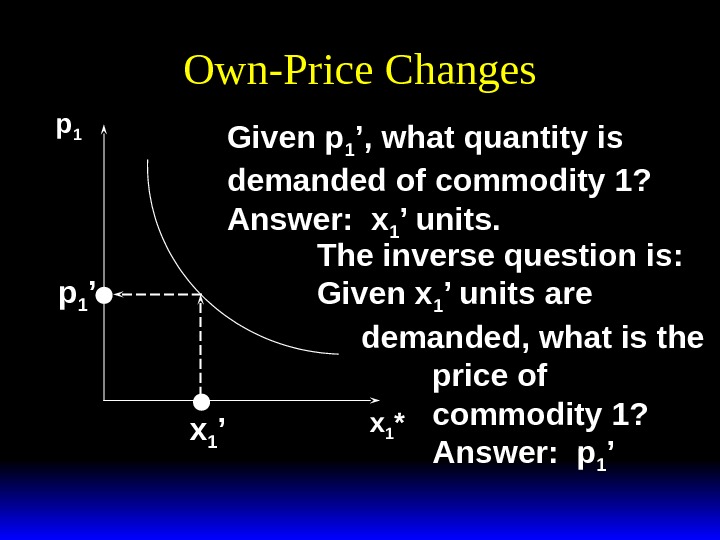
Own-Price Changes Usually we ask “Given the price for commodity 1 what is the quantity demanded of commodity 1? ” But we could also ask the inverse question “At what price for commodity 1 would a given quantity of commodity 1 be demanded? ”

Own-Price Changes p 1 x 1 *p 1 ’ Given p 1 ’, what quantity is demanded of commodity 1?

Own-Price Changes p 1 x 1 *p 1 ’ Given p 1 ’, what quantity is demanded of commodity 1? Answer: x 1 ’ units. x 1 ’

Own-Price Changes p 1 x 1 * x 1 ’ Given p 1 ’, what quantity is demanded of commodity 1? Answer: x 1 ’ units. The inverse question is: Given x 1 ’ units are demanded, what is the price of commodity 1?

Own-Price Changes p 1 x 1 *p 1 ’ x 1 ’ Given p 1 ’, what quantity is demanded of commodity 1? Answer: x 1 ’ units. The inverse question is: Given x 1 ’ units are demanded, what is the price of commodity 1? Answer: p 1 ’

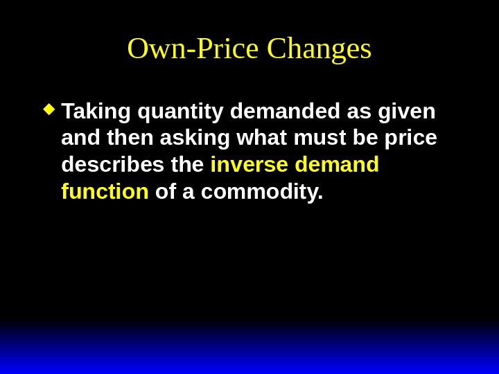
Own-Price Changes Taking quantity demanded as given and then asking what must be price describes the inverse demand function of a commodity.

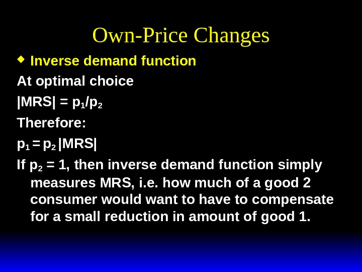
Own-Price Changes Inverse demand function At optimal choice |MRS| = p 1 /p 2 Therefore: p 1 = p 2 |MRS| If p 2 = 1, then inverse demand function simply measures MRS, i. e. how much of a good 2 consumer would want to have to compensate for a small reduction in amount of good 1.

Own-Price Changes Inverse demand function If good 2 is money, then MRS (and inverse demand function) measure marginal willingness to pay.

Own-Price Changes A Cobb-Douglas example: x ay abp 1 1 * () is the ordinary demand function and p ay abx 1 1 () * is the inverse demand function.

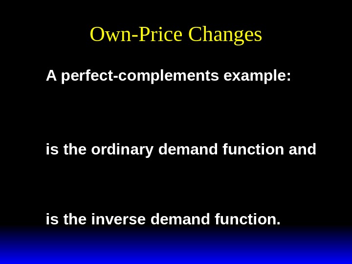
Own-Price Changes A perfect-complements example: x y pp 1 12 * is the ordinary demand function and p y x p 1 1 2 * is the inverse demand function.

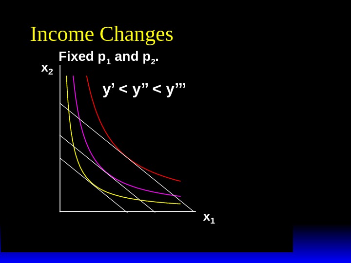
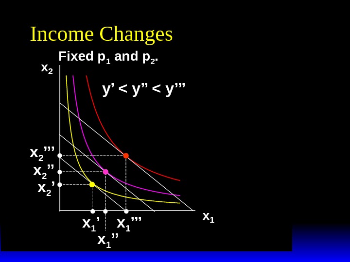
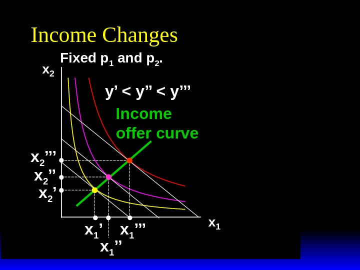
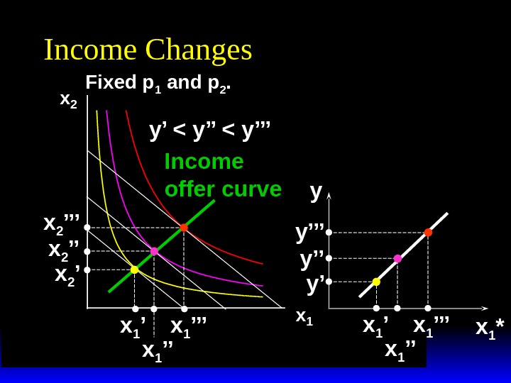
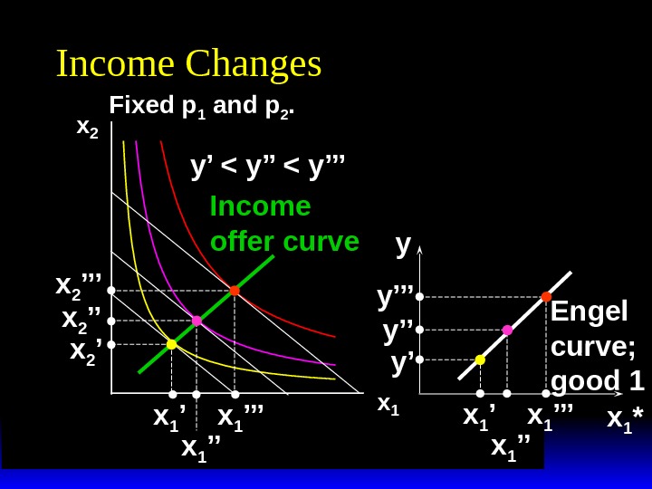
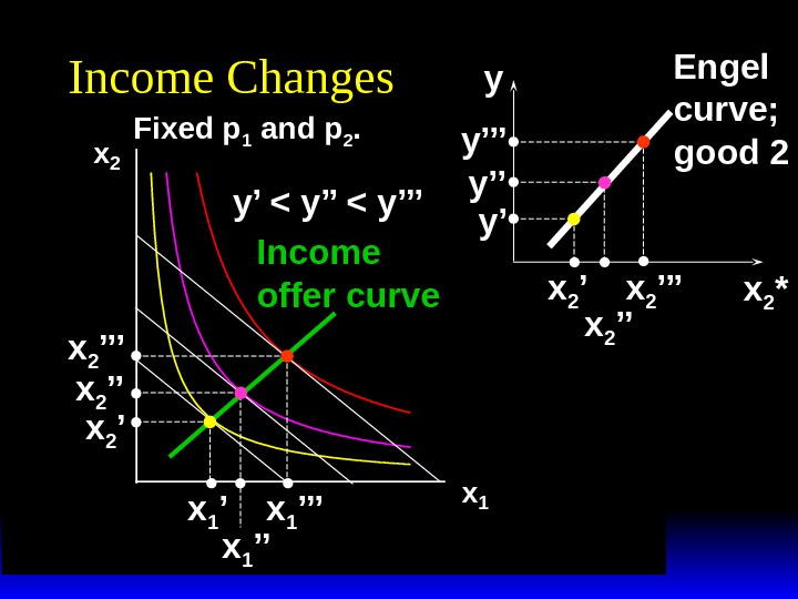
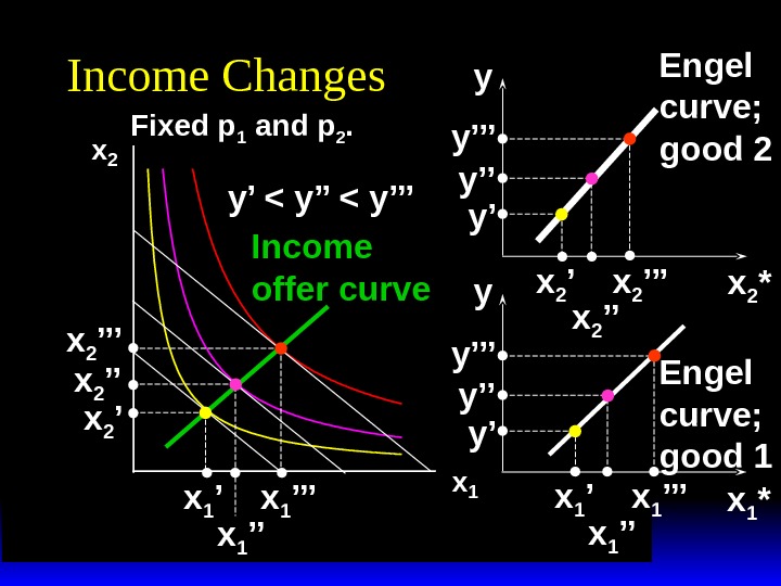
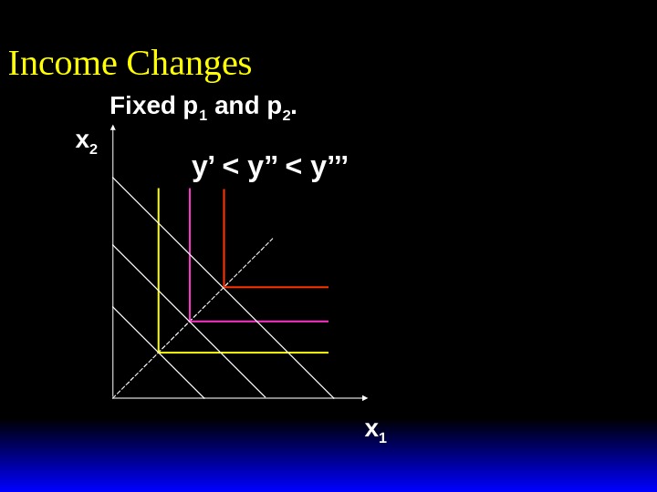
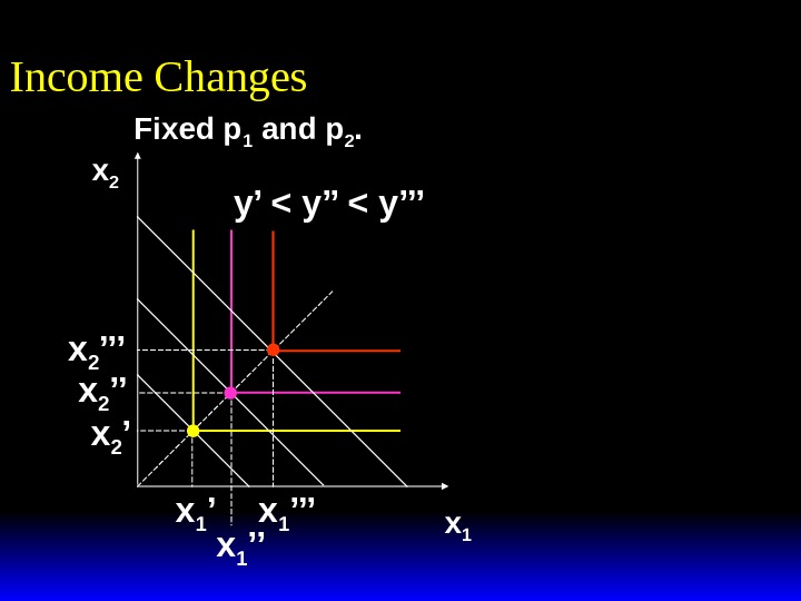
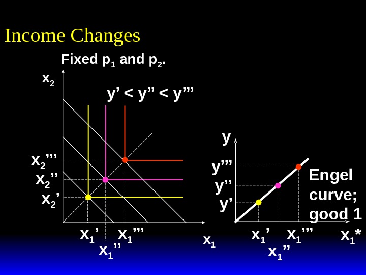
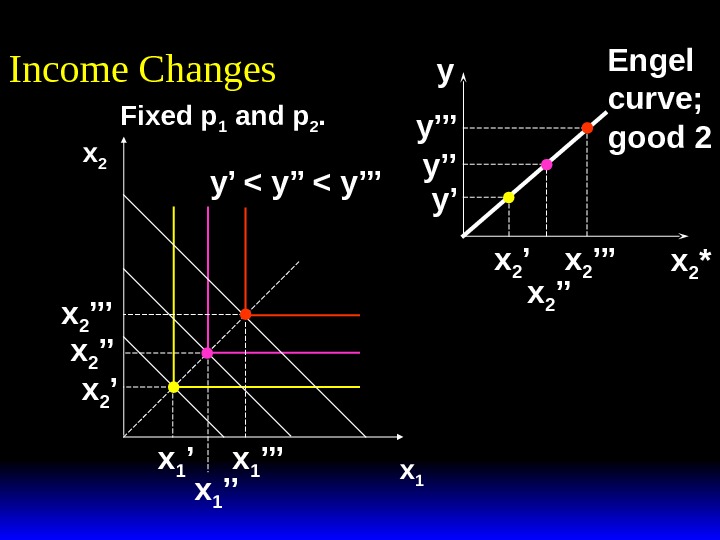
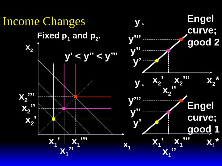
Income Changes How does the value of x 1 *(p 1 , p 2 , y) change as y changes, holding both p 1 and p 2 constant?

x 2 x 1 Income Changes Fixed p 1 and p 2. y’ < y’’’

x 2 x 1 Income Changes Fixed p 1 and p 2. y’ < y’’’

x 2 x 1 Income Changes Fixed p 1 and p 2. y’ < y’’’ x 1 ’’x 1 ’x 2 ’’’ x 2 ’

x 2 x 1 Income Changes Fixed p 1 and p 2. y’ < y’’’ x 1 ’’x 1 ’x 2 ’’’ x 2 ’ Income offer curve

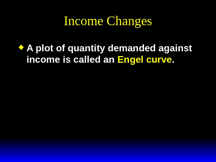
Income Changes A plot of quantity demanded against income is called an Engel curve.

x 2 x 1 Income Changes Fixed p 1 and p 2. y’ < y’’’ x 1 ’’x 1 ’x 2 ’’’ x 2 ’ Income offer curve

x 2 x 1 Income Changes Fixed p 1 and p 2. y’ < y’’’ x 1 ’’x 1 ’x 2 ’’’ x 2 ’ Income offer curve x 1 *y x 1 ’’’ x 1 ’’x 1 ’y’y’’y’’’

x 2 x 1 Income Changes Fixed p 1 and p 2. y’ < y’’’ x 1 ’’x 1 ’x 2 ’’’ x 2 ’ Income offer curve x 1 *y x 1 ’’’ x 1 ’’x 1 ’y’y’’y’’’ Engel curve; good

x 2 x 1 Income Changes Fixed p 1 and p 2. y’ < y’’’ x 1 ’’x 1 ’x 2 ’’’ x 2 ’ Income offer curve x 2 *y x 2 ’’’ x 2 ’’x 2 ’y’y’’y’’’

x 2 x 1 Income Changes Fixed p 1 and p 2. y’ < y’’’ x 1 ’’x 1 ’x 2 ’’’ x 2 ’ Income offer curve x 2 *y x 2 ’’’ x 2 ’’x 2 ’y’y’’y’’’ Engel curve; good

x 2 x 1 Income Changes Fixed p 1 and p 2. y’ < y’’’ x 1 ’’x 1 ’x 2 ’’’ x 2 ’ Income offer curve x 1 *x 2 *y y x 1 ’’’ x 1 ’’x 1 ’ x 2 ’’x 2 ’y’y’’y’’’ Engel curve; good 2 Engel curve; good

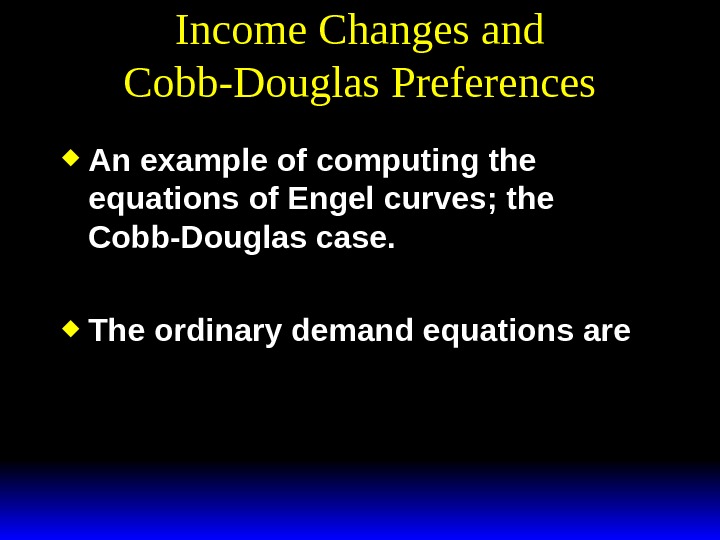
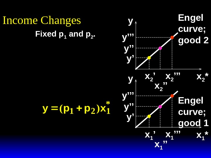
Income Changes and Cobb-Douglas Preferences An example of computing the equations of Engel curves; the Cobb-Douglas case. The ordinary demand equations are. Uxxxx ab (, ). 1212 x ay abp x by abp 1 1 2 2 ** () ; ().

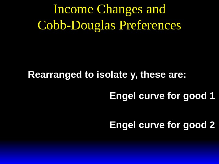
Income Changes and Cobb-Douglas Preferencesx ay abp x by abp 1 1 2 2 ** () ; (). Rearranged to isolate y, these are: y abp a x y abp b x () () * * 1 1 2 2 Engel curve for good 1 Engel curve for good

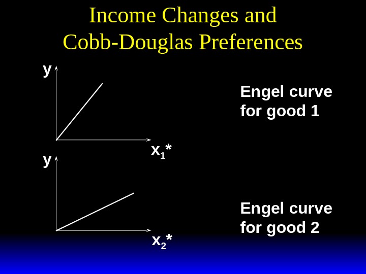
Income Changes and Cobb-Douglas Preferences y y x 1 * x 2 *y abp a x ()*1 1 Engel curve for good 1 y abp b x ()*2 2 Engel curve for good

Income Changes and Perfectly-Complementary Preferences Another example of computing the equations of Engel curves; the perfectly-complementary case. The ordinary demand equations arexx y pp 12 12 **. Uxxxx(, )min, .

Income Changes and Perfectly-Complementary Preferences Rearranged to isolate y, these are: yppx () () * * 121 122 Engel curve for good 1 xx y pp 12 12 **. Engel curve for good

Fixed p 1 and p 2. Income Changes x 1 x

Income Changes x 1 x 2 y’ < y’’’Fixed p 1 and p 2.

Income Changes x 1 x 2 y’ < y’’’Fixed p 1 and p 2.

Income Changes x 1 x 2 y’ < y’’’ x 1 ’’x 1 ’x 2 ’’’ x 2 ’ x 1 ’’’Fixed p 1 and p 2.

Income Changes x 1 x 2 y’ < y’’’ x 1 ’’x 1 ’x 2 ’’’ x 2 ’ x 1 ’’’ x 1 *y y’y’’y’’’ Engel curve; good 1 x 1 ’’’ x 1 ’’x 1 ’Fixed p 1 and p 2.

Income Changes x 1 x 2 y’ < y’’’ x 1 ’’x 1 ’x 2 ’’’ x 2 ’ x 1 ’’’ x 2 *y x 2 ’’’ x 2 ’’x 2 ’y’y’’y’’’ Engel curve; good 2 Fixed p 1 and p 2.

Income Changes x 1 x 2 y’ < y’’’ x 1 ’’x 1 ’x 2 ’’’ x 2 ’ x 1 ’’’ x 1 *x 2 *y y x 2 ’’’ x 2 ’’x 2 ’y’y’’y’’’ Engel curve; good 2 Engel curve; good 1 x 1 ’’’ x 1 ’’x 1 ’Fixed p 1 and p 2.

Income Changes x 1 *x 2 *y y x 2 ’’’ x 2 ’’x 2 ’y’y’’y’’’ x 1 ’’x 1 ’yppx() * 122 yppx() * 121 Engel curve; good 2 Engel curve; good 1 Fixed p 1 and p 2.

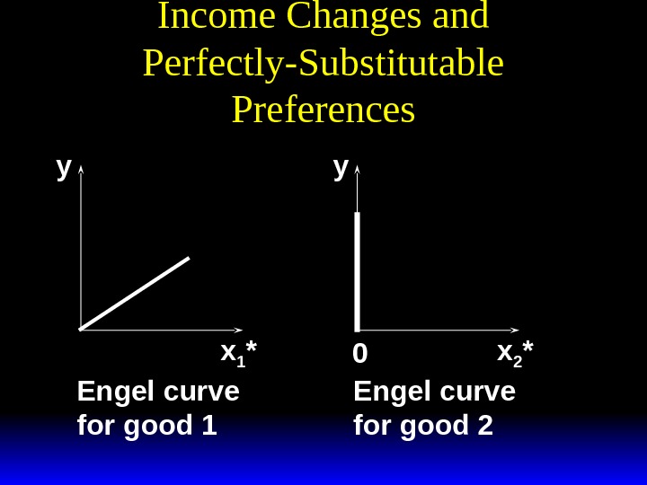
Income Changes and Perfectly-Substitutable Preferences Another example of computing the equations of Engel curves; the perfectly-substitution case. The ordinary demand equations are. Uxxxx(, ).

Income Changes and Perfectly-Substitutable Preferencesxppy ifpp ypifpp 112 12 112 0 * (, , ) , /, xppy ifpp ypifpp 212 12 212 0 * (, , ) , /, .

Income Changes and Perfectly-Substitutable Preferencesxppy ifpp ypifpp 112 12 112 0 * (, , ) , /, xppy ifpp ypifpp 212 12 212 0 * (, , ) , /, . Suppose p 1 < p 2. Then

Income Changes and Perfectly-Substitutable Preferencesxppy ifpp ypifpp 112 12 112 0 * (, , ) , /, xppy ifpp ypifpp 212 12 212 0 * (, , ) , /, . Suppose p 1 < p 2. Then x y p 1 1 * x 20 * and

Income Changes and Perfectly-Substitutable Preferencesxppy ifpp ypifpp 112 12 112 0 * (, , ) , /, xppy ifpp ypifpp 212 12 212 0 * (, , ) , /, . Suppose p 1 < p 2. Then x y p 1 1 * x 20 * and x 20 *. ypx 11 * and

Income Changes and Perfectly-Substitutable Preferencesx 20 *. ypx 11 * y y x 1 * x 2 * 0 Engel curve for good 1 Engel curve for good

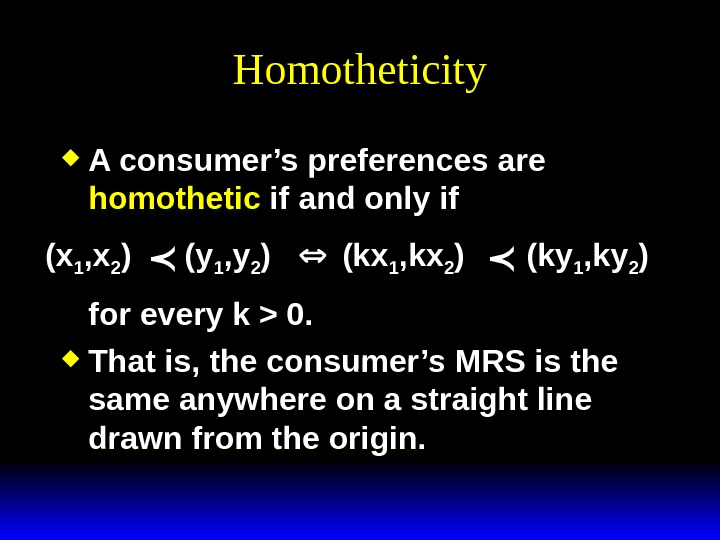
Income Changes In every example so far the Engel curves have all been straight lines? Q: Is this true in general? A: No. Engel curves are straight lines if the consumer’s preferences are homothetic.

Homotheticity A consumer’s preferences are homothetic if and only if for every k > 0. That is, the consumer’s MRS is the same anywhere on a straight line drawn from the origin. (x 1 , x 2 ) (y 1 , y 2 ) (kx 1 , kx 2 ) (ky 1 , ky 2 )

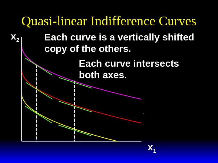
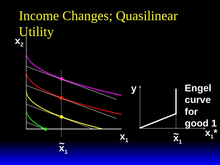
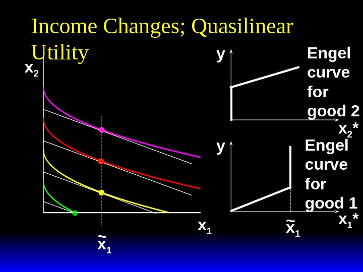
Income Effects — A Nonhomothetic Example Quasilinear preferences are not homothetic. For example, Uxxfxx(, )(). 1212 Uxxxx(, ).

Quasi-linear Indifference Curves x 2 x 1 Each curve is a vertically shifted copy of the others. Each curve intersects both axes.

Income Changes; Quasilinear Utility x 2 x 1~

Income Changes; Quasilinear Utility x 2 x 1~ x 1 *y x 1~ Engel curve for good

Income Changes; Quasilinear Utility x 2 x 1~ x 2 *y Engel curve for good

Income Changes; Quasilinear Utility x 2 x 1~ x 1 *x 2 * yy x 1~ Engel curve for good 2 Engel curve for good

Income Effects A good for which quantity demanded rises with income is called normal. Therefore a normal good’s Engel curve is positively sloped.

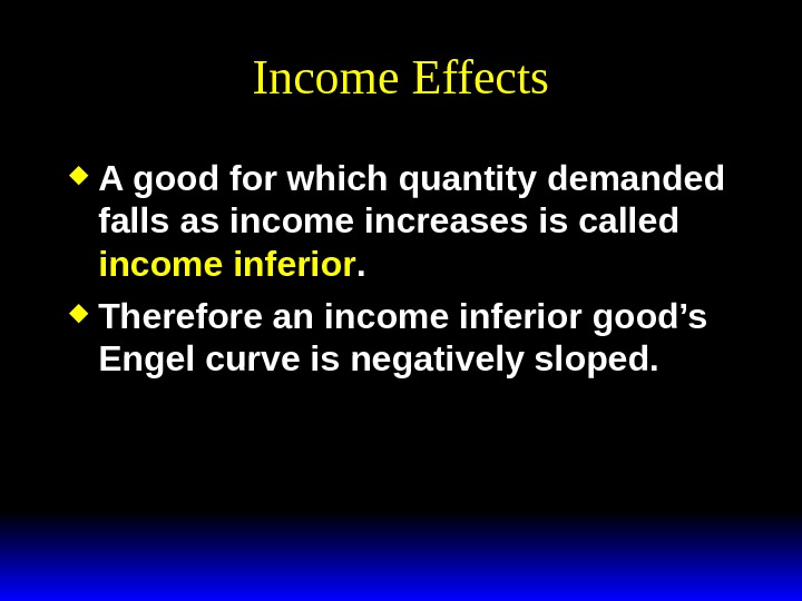
Income Effects A good for which quantity demanded falls as income increases is called income inferior. Therefore an income inferior good’s Engel curve is negatively sloped.

Income Effects In the US over last hundred years income increased many times whereas the number of kids per household went down. A re children an inferior good?

x 2 x 1 Income Changes; Goods 1 & 2 Normal x 1 ’’’ x 1 ’’x 1 ’x 2 ’’’ x 2 ’ Income offer curve x 1 *x 2 *y y x 1 ’’’ x 1 ’’x 1 ’ x 2 ’’x 2 ’y’y’’y’’’ Engel curve; good 2 Engel curve; good

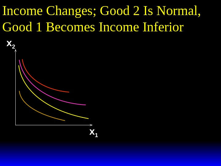
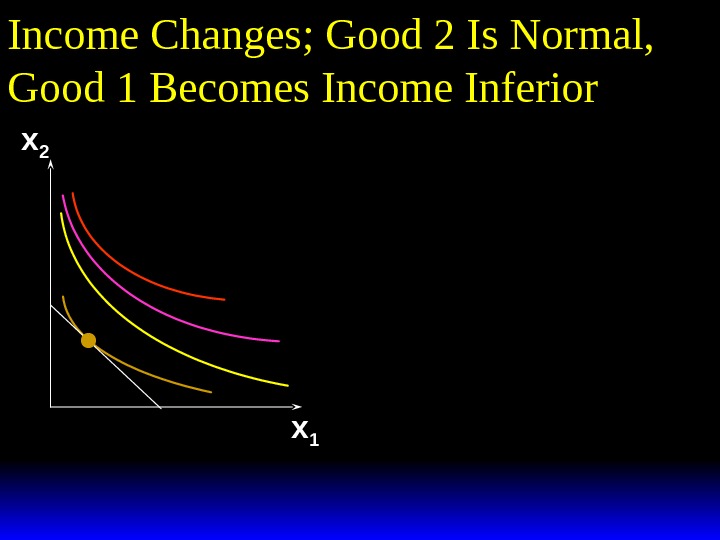
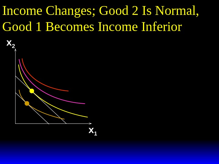
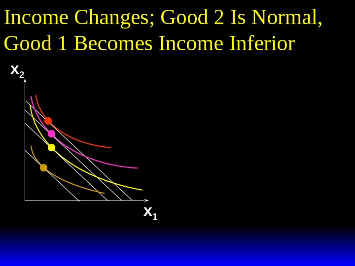
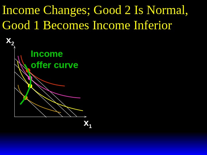
Income Changes; Good 2 Is Normal, Good 1 Becomes Income Inferior x 2 x

Income Changes; Good 2 Is Normal, Good 1 Becomes Income Inferior x 2 x

Income Changes; Good 2 Is Normal, Good 1 Becomes Income Inferior x 2 x

Income Changes; Good 2 Is Normal, Good 1 Becomes Income Inferior x 2 x

Income Changes; Good 2 Is Normal, Good 1 Becomes Income Inferior x 2 x

Income Changes; Good 2 Is Normal, Good 1 Becomes Income Inferior x 2 x 1 Income offer curve

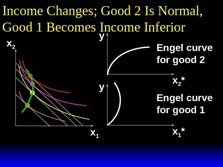
Income Changes; Good 2 Is Normal, Good 1 Becomes Income Inferior x 2 x 1 *y Engel curve for good

Income Changes; Good 2 Is Normal, Good 1 Becomes Income Inferior x 2 x 1 *x 2 *y y Engel curve for good 2 Engel curve for good

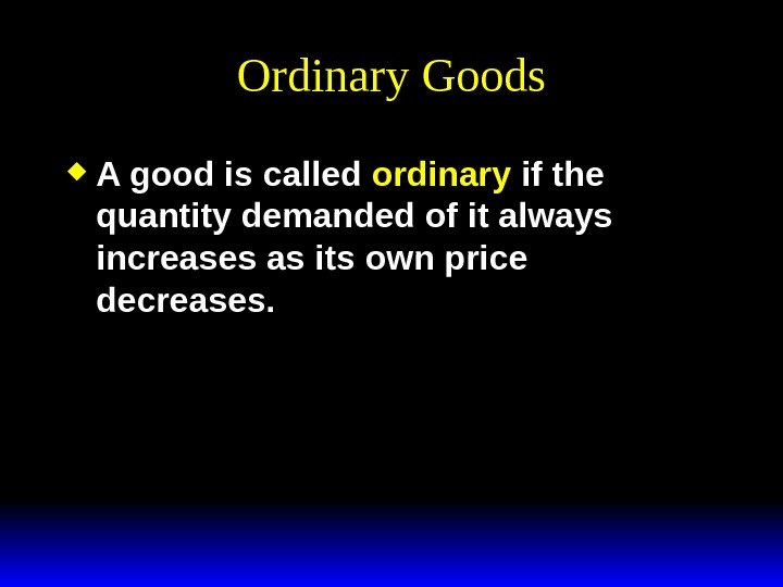
Ordinary Goods A good is called ordinary if the quantity demanded of it always increases as its own price decreases.

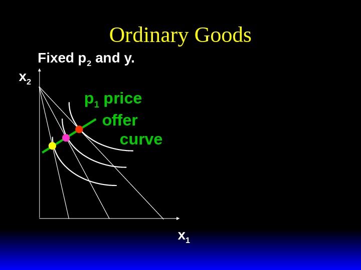
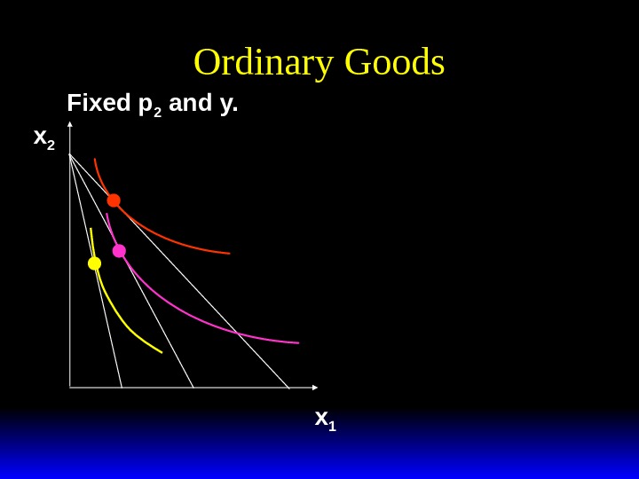
Ordinary Goods Fixed p 2 and y. x 1 x

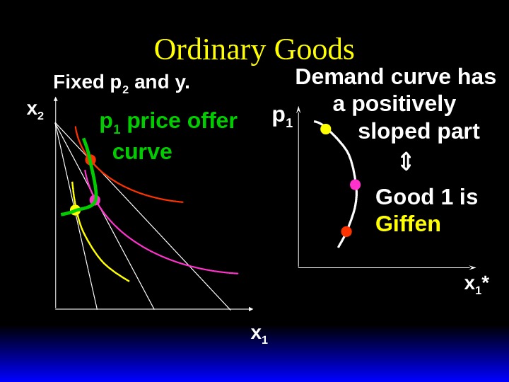
Ordinary Goods Fixed p 2 and y. x 1 x 2 p 1 price offer curve

Ordinary Goods Fixed p 2 and y. x 1 x 2 p 1 price offer curve x 1 *Downward-sloping demand curve Good 1 is ordinaryp

Giffen Goods If, for some values of its own price, the quantity demanded of a good rises as its own-price increases then the good is called Giffen.

Ordinary Goods Fixed p 2 and y. x 1 x

Ordinary Goods Fixed p 2 and y. x 1 x 2 p 1 price offer curve

Ordinary Goods Fixed p 2 and y. x 1 x 2 p 1 price offer curve x 1 *Demand curve has a positively sloped part Good 1 is Giffenp

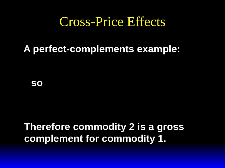
Cross-Price Effects If an increase in p 2 – increases demand for commodity 1 then commodity 1 is a gross substitute for commodity 2. – reduces demand for commodity 1 then commodity 1 is a gross complement for commodity 2.

Cross-Price Effects A perfect-complements example: x y pp 1 12 * x p y pp 1 212 2 0 *. so Therefore commodity 2 is a gross complement for commodity 1.

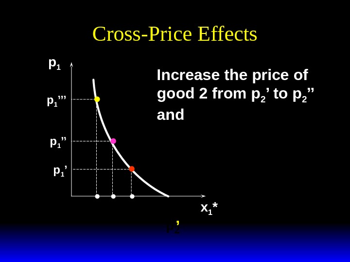
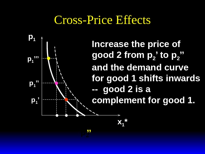
Cross-Price Effects p 1 x 1 *p 1 ’’p 1 ’’’y p 2 ’Increase the price of good 2 from p 2 ’ to p 2 ’’ and

Cross-Price Effects p 1 x 1 *p 1 ’’p 1 ’’’y p 2 ’’ Increase the price of good 2 from p 2 ’ to p 2 ’’ and the demand curve for good 1 shifts inwards — good 2 is a complement for good 1.

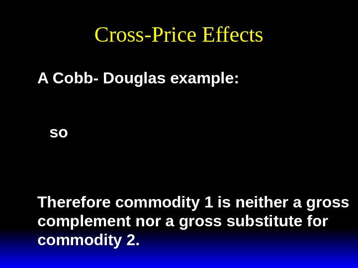
Cross-Price Effects A Cobb- Douglas example: x by abp 2 2 * () so

Cross-Price Effects A Cobb- Douglas example: x by abp 2 2 * () x p 2 1 0 *. so Therefore commodity 1 is neither a gross complement nor a gross substitute for commodity 2.