Business Microeconomics Instructor: Gulnara Moldasheva 1 Perfect Competition

Business Microeconomics Instructor: Gulnara Moldasheva 1 Perfect Competition CHAPTER

Business Microeconomics Instructor: Gulnara Moldasheva

Business Microeconomics Instructor: Gulnara Moldasheva 3 Airlines and automobile producers are facing tough times: Prices are being slashed to drive sales and profits are turning into losses. Workers have been laid off temporarily or let go permanently. What determines the firm’s price and profit? Why do firms sometimes stop producing and temporarily lay off their workers? To study competitive markets, we are going to build a model of a market in which competition is as fierce and extreme as. We call this situation “perfect competition. ”

Business Microeconomics Instructor: Gulnara Moldasheva 4 What Is Perfect Competition? Perfect competition is an industry in which Many firms sell identical products to many buyers. There are no restrictions to entry into the industry. Established firms have no advantages over new ones. Sellers and buyers are well informed about prices.

Business Microeconomics Instructor: Gulnara Moldasheva 5 How Perfect Competition Arises Perfect competition arises: When firm’s minimum efficient scale is small relative to market demand so there is room for many firms in the industry. And when each firm is perceived to produce a good or service that has no unique characteristics, so consumers don’t care which firm they buy from. What Is Perfect Competition?

Business Microeconomics Instructor: Gulnara Moldasheva 6 Price Takers In perfect competition, each firm is a price taker. A price taker is a firm that cannot influence the price of a good or service. No single firm can influence the price—it must “take” the equilibrium market price. Each firm’s output is a perfect substitute for the output of the other firms, so the demand for each firm’s output is perfectly elastic. What Is Perfect Competition?

Business Microeconomics Instructor: Gulnara Moldasheva 7 Economic Profit and Revenue The goal of each firm is to maximize economic profit , which equals total revenue minus total cost. Total cost is the opportunity cost of production, which includes normal profit. A firm’s total revenue equals price, P , multiplied by quantity sold, Q , or P × Q. A firm’s marginal revenue is the change in total revenue that results from a one-unit increase in the quantity sold. What Is Perfect Competition?

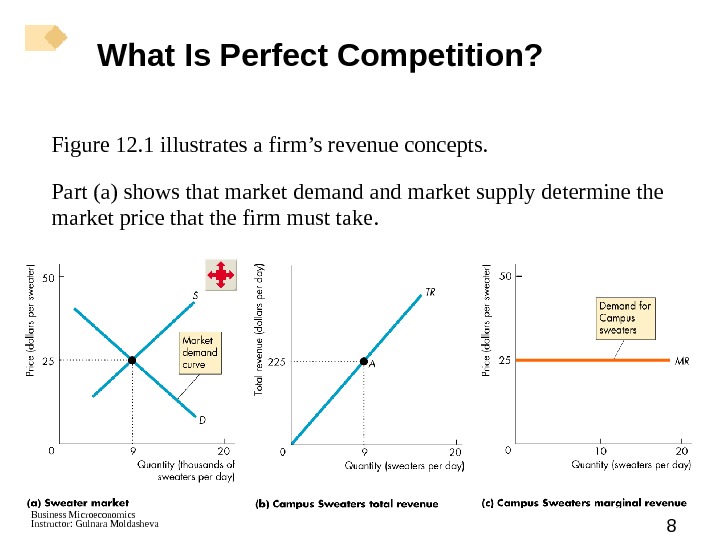
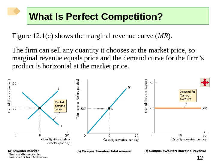
Business Microeconomics Instructor: Gulnara Moldasheva 8 Figure 12. 1 illustrates a firm’s revenue concepts. Part (a) shows that market demand market supply determine the market price that the firm must take. What Is Perfect Competition?

Business Microeconomics Instructor: Gulnara Moldasheva 10 Figure 12. 1(b) shows the firm’s total revenue curve ( TR )—the relationship between total revenue and quantity sold. What Is Perfect Competition?

Business Microeconomics Instructor: Gulnara Moldasheva 12 Figure 12. 1(c) shows the marginal revenue curve ( MR ). The firm can sell any quantity it chooses at the market price, so marginal revenue equals price and the demand curve for the firm’s product is horizontal at the market price. What Is Perfect Competition?

Business Microeconomics Instructor: Gulnara Moldasheva 14 The demand for a firm’s product is perfectly elastic because one firm’s sweater is a perfect substitute for the sweater of another firm. The market demand is not perfectly elastic because a sweater is a substitute for some other good. What Is Perfect Competition?

Business Microeconomics Instructor: Gulnara Moldasheva 15 A perfectly competitive firm’s goal is to make maximum economic profit, given the constraints it faces. So the firm must decide: 1. How to produce at minimum cost 2. What quantity to produce 3. Whether to enter or exit a market We start by looking at the firm’s output decision. What Is Perfect Competition?

Business Microeconomics Instructor: Gulnara Moldasheva 16 Profit-Maximizing Output A perfectly competitive firm chooses the output that maximizes its economic profit. One way to find the profit-maximizing output is to look at the firm’s the total revenue and total cost curves. Figure 12. 2 on the next slide looks at these curves along with the firm’s total profit curve. The Firm’s Output Decision

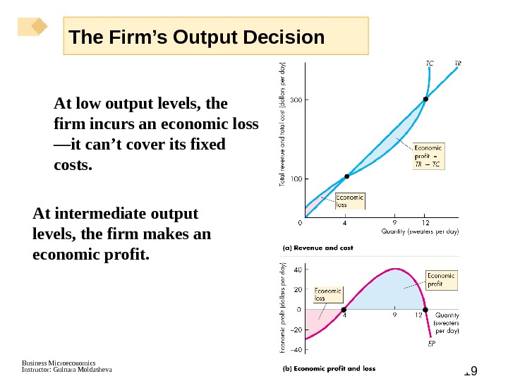
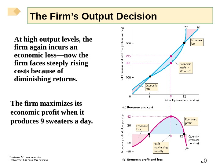
Business Microeconomics Instructor: Gulnara Moldasheva 17 Part (a) shows the total revenue, TR , curve. Part (a) also shows the total cost curve, TC , which is like the one in Chapter 11. Total revenue minus total cost is economic profit (or loss), shown by the curve EP in part (b). The Firm’s Output Decision

Business Microeconomics Instructor: Gulnara Moldasheva 19 At low output levels, the firm incurs an economic loss —it can’t cover its fixed costs. At intermediate output levels, the firm makes an economic profit. The Firm’s Output Decision

Business Microeconomics Instructor: Gulnara Moldasheva 20 At high output levels, the firm again incurs an economic loss—now the firm faces steeply rising costs because of diminishing returns. The firm maximizes its economic profit when it produces 9 sweaters a day. The Firm’s Output Decision

Business Microeconomics Instructor: Gulnara Moldasheva 21 Marginal Analysis and Supply Decision The firm can use marginal analysis to determine the profit-maximizing output. Because marginal revenue is constant and marginal cost eventually increases as output increases, profit is maximized by producing the output at which marginal revenue, MR , equals marginal cost, MC. Figure 12. 3 on the next slide shows the marginal analysis that determines the profit-maximizing output. The Firm’s Output Decision

Business Microeconomics Instructor: Gulnara Moldasheva 22 If MR > MC , economic profit increases if output increases. If MR < MC , economic profit decreases if output increases. If MR = MC , economic profit decreases if output changes in either direction, so economic profit is maximized. The Firm’s Output Decision

Business Microeconomics Instructor: Gulnara Moldasheva 24 Temporary Shutdown Decision If the firm makes an economic loss it must decide to exit the market or to stay in the market. If the firm decides to stay in the market, it must decide whether to produce something or to shut down temporarily. The decision will be the one that minimizes the firm’s loss. The Firm’s Output Decision

Business Microeconomics Instructor: Gulnara Moldasheva 25 Loss Comparison The firm’s loss equals total fixed cost ( TFC ) plus total variable cost ( TVC ) minus total revenue ( TR ). Economic loss = TFC + TVC TR = TFC + (AVC P ) × Q If the firm shuts down, Q is 0 and the firm still has to pay its TFC. So the firm incurs an economic loss equal to TFC. This economic loss is the largest that the firm must bear. The Firm’s Output Decision

Business Microeconomics Instructor: Gulnara Moldasheva 26 A firm’s shutdown point is the price and quantity at which it is indifferent between producing and shutting down. This point is where AVC is at its minimum. It is also the point at which the MC curve crosses the AVC curve. At the shutdown point, the firm is indifferent between producing and shutting down temporarily. The firm incurs a loss equal to TFC from either action. The Firm’s Output Decision

Business Microeconomics Instructor: Gulnara Moldasheva 27 Figure 12. 4 shows the shutdown point. Minimum AVC is $17 a sweater. If the price is $17, the profit-maximizing output is 7 sweaters a day. The firm incurs a loss equal to the red rectangle. The Firm’s Output Decision

Business Microeconomics Instructor: Gulnara Moldasheva 29 If the price of a sweater is between $17 and $20. 14, the firm produces the quantity at which marginal cost equals price. The firm covers all its variable cost and at least part of its fixed cost. It incurs a loss that is less than TFC. The Firm’s Output Decision

Business Microeconomics Instructor: Gulnara Moldasheva 30 The Firm’s Supply Curve A perfectly competitive firm’s supply curve shows how the firm’s profit-maximizing output varies as the market price varies, other things remaining the same. Because the firm produces the output at which marginal cost equals marginal revenue, and because marginal revenue equals price, the firm’s supply curve is linked to its marginal cost curve. But at a price below the shutdown point, the firm produces nothing. The Firm’s Output Decision

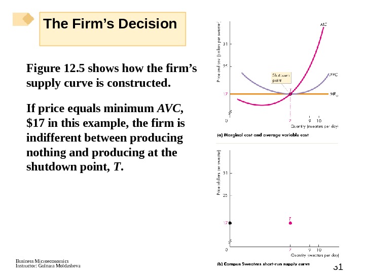
Business Microeconomics Instructor: Gulnara Moldasheva 31 Figure 12. 5 shows how the firm’s supply curve is constructed. If price equals minimum AVC , $17 in this example, the firm is indifferent between producing nothing and producing at the shutdown point, T. The Firm’s Decision

Business Microeconomics Instructor: Gulnara Moldasheva 33 If the price is $25, the firm produces 9 sweaters a day, the quantity at which P = MC. If the price is $31, the firm produces 10 sweaters a day, the quantity at which P = MC. The blue curve in part (b) traces the firm’s short-run supply curve. The Firm’s Decisions

Business Microeconomics Instructor: Gulnara Moldasheva 34 Market Supply in the Short Run The short-run market supply curve shows the quantity supplied by all firms in the market at each price when each firm’s plant and the number of firms remain the same. Output, Price, and Profit in the Short Run

Business Microeconomics Instructor: Gulnara Moldasheva 35 Figure 12. 6 shows the supply curve for a market that has 1, 000 firms like Campus Sweaters. The quantity supplied by the market at any given price is the sum of the quantities supplied by all the firms in the market at that price. Output, Price, and Profit in the Short Run

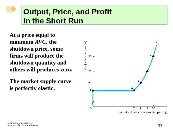
Business Microeconomics Instructor: Gulnara Moldasheva 37 At a price equal to minimum AVC, the shutdown price , some firms will produce the shutdown quantity and others will produces zero. The market supply curve is perfectly elastic. Output, Price, and Profit in the Short Run

Business Microeconomics Instructor: Gulnara Moldasheva 38 Short-Run Equilibrium Short-run market supply and market demand determine the market price and output. Figure 12. 7 shows a short-run equilibrium. Output, Price, and Profit in the Short Run

Business Microeconomics Instructor: Gulnara Moldasheva 40 A Change in Demand An increase in demand bring a rightward shift of the market demand curve: The price rises and the quantity increases. A decrease in demand bring a leftward shift of the market demand curve: The price falls and the quantity decreases. Output, Price, and Profit in the Short Run

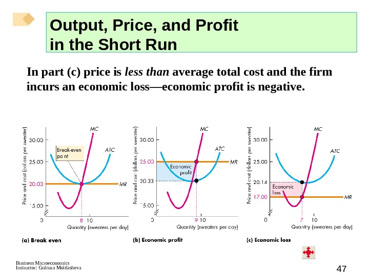
Business Microeconomics Instructor: Gulnara Moldasheva 42 Profits and Losses in the Short Run Maximum profit is not always a positive economic profit. To determine whether a firm is making an economic profit or incurring an economic loss, we compare the firm’s average total cost at the profit-maximizing output with the market price. Figure 12. 8 on the next slide shows the three possible profit outcomes. Output, Price, and Profit in the Short Run

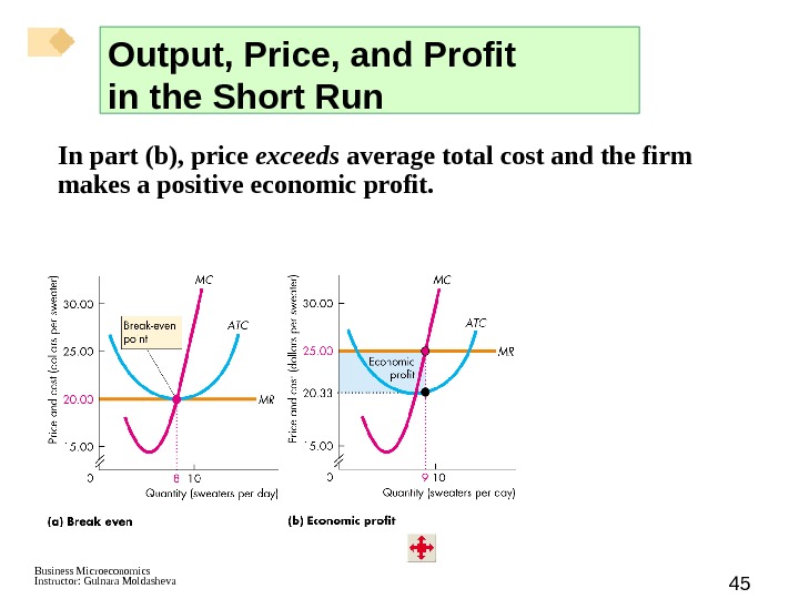
Business Microeconomics Instructor: Gulnara Moldasheva 43 In part (a) price equals average total cost and the firm makes zero economic profit (breaks even). Output, Price, and Profit in the Short Run

Business Microeconomics Instructor: Gulnara Moldasheva 45 In part (b), price exceeds average total cost and the firm makes a positive economic profit. Output, Price, and Profit in the Short Run

Business Microeconomics Instructor: Gulnara Moldasheva 47 In part (c) price is less than average total cost and the firm incurs an economic loss—economic profit is negative. Output, Price, and Profit in the Short Run

Business Microeconomics Instructor: Gulnara Moldasheva 49 In short-run equilibrium, a firm may make an economic profit, break even, or incur an economic loss. Only one of them is a long-run equilibrium because firms can enter or exit the market. Output, Price, and Profit in the Long Run

Business Microeconomics Instructor: Gulnara Moldasheva 50 Entry and Exit New firms enter an industry in which existing firms make an economic profit. Firms exit an industry in which they incur an economic loss. Figure 12. 8 shows the effects of entry and exit. Output, Price, and Profit in the Long Run

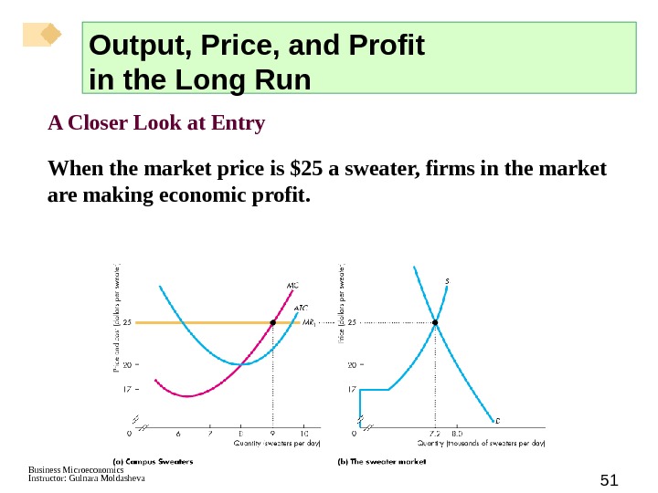
Business Microeconomics Instructor: Gulnara Moldasheva 51 A Closer Look at Entry When the market price is $25 a sweater, firms in the market are making economic profit. Output, Price, and Profit in the Long Run

Business Microeconomics Instructor: Gulnara Moldasheva 53 New firms have an incentive to enter the market. When they do, the market supply increases and the market price falls. Output, Price, and Profit in the Long Run

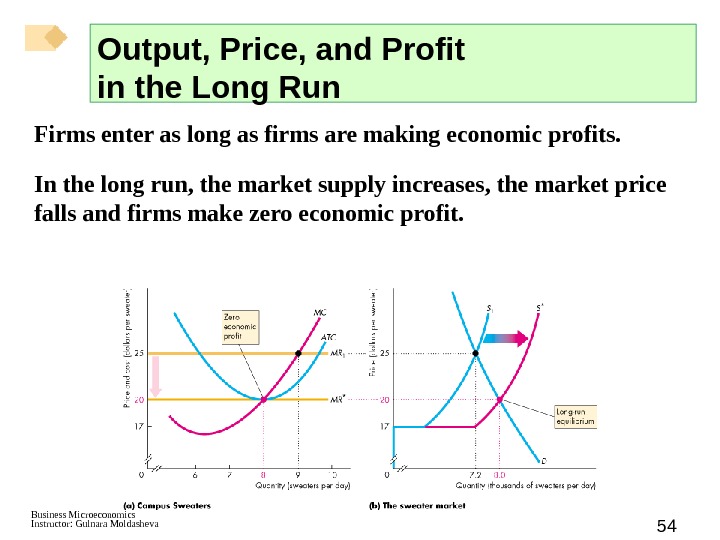
Business Microeconomics Instructor: Gulnara Moldasheva 54 Firms enter as long as firms are making economic profits. In the long run, the market supply increases, the market price falls and firms make zero economic profit. Output, Price, and Profit in the Long Run

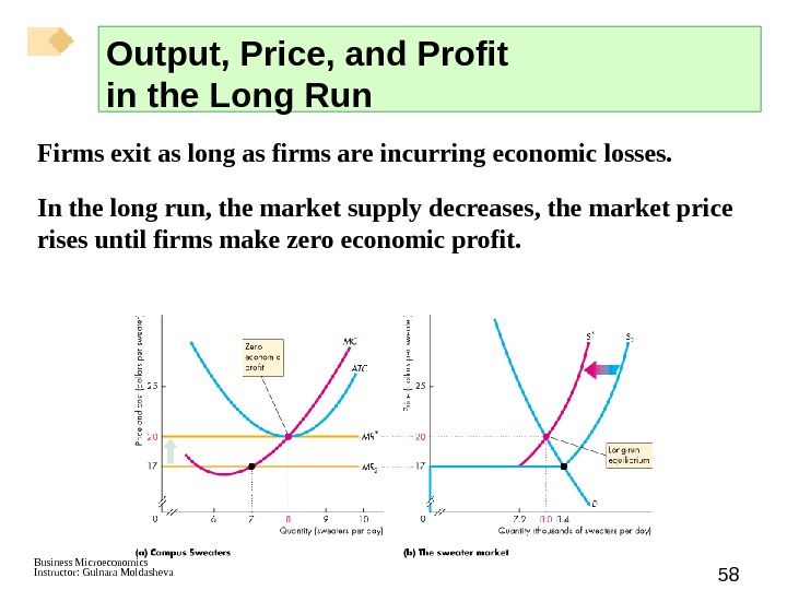
Business Microeconomics Instructor: Gulnara Moldasheva 55 A Closer Look at Exit When the market price is $17 a sweater, firms in the market are incurring economic loss. Output, Price, and Profit in the Long Run

Business Microeconomics Instructor: Gulnara Moldasheva 58 Firms exit as long as firms are incurring economic losses. In the long run, the market supply decreases, the market price rises until firms make zero economic profit. Output, Price, and Profit in the Long Run

Business Microeconomics Instructor: Gulnara Moldasheva 59 Changing Tastes and Advancing Technology A Permanent Change in Demand A decrease in demand shifts the market demand curve leftward. The price falls and the quantity decreases. Figure 12. 10 illustrates the effects of a permanent decrease in demand when the market is in long-run equilibrium.

Business Microeconomics Instructor: Gulnara Moldasheva 60 A decrease in demand shifts the market demand curve leftward. The market price falls, and each firm decreases the quantity it produces. Changing Tastes and Advancing Technology

Business Microeconomics Instructor: Gulnara Moldasheva 62 The market price is now below each firm’s minimum average total cost, so firms incur economic losses. Changing Tastes and Advancing Technology

Business Microeconomics Instructor: Gulnara Moldasheva 63 Economic losses induce some firms to exit in the long run, which decreases the market supply and the price starts to rise. Changing Tastes and Advancing Technology

Business Microeconomics Instructor: Gulnara Moldasheva 64 As the price rises, the quantity produced by all firms continues to decrease as more firms exit, but each firm remaining in the market starts to increase its quantity. Changing Tastes and Advancing Technology

Business Microeconomics Instructor: Gulnara Moldasheva 65 A new long-run equilibrium occurs when the price has risen to equal minimum average total cost. Firms make zero economic profits, and firms no longer exit the market. Changing Tastes and Advancing Technology

Business Microeconomics Instructor: Gulnara Moldasheva 66 The main difference between the initial and new long-run equilibrium is the number of firms in the market. Fewer firms produce the equilibrium quantity. Changing Tastes and Advancing Technology

Business Microeconomics Instructor: Gulnara Moldasheva 67 A permanent increase in demand has the opposite effects to those just described and shown in Figure 12. 10. A permanent increase in demand shifts the demand curve rightward. The price rises and the quantity increases. Economic profit induces entry, which increases short-run supply and shifts the short-run market supply curve rightward. As the market supply increases, the price falls and the market quantity continues to increase. Changing Tastes and Advancing Technology

Business Microeconomics Instructor: Gulnara Moldasheva 68 With a falling price, each firm decreases its output as it moves along its marginal cost curve (supply curve). A new long-run equilibrium occurs when the price has fallen to equal minimum average total cost. Firms make zero economic profit, and firms have no incentive to enter the market. The main difference between the initial and new long-run equilibrium is the number of firms. In the new equilibrium, a larger number of firms produce the equilibrium quantity. Changing Tastes and Advancing Technology

Business Microeconomics Instructor: Gulnara Moldasheva 69 External Economics and Diseconomies The change in the long-run equilibrium price following a permanent change in demand depends on external economies and external diseconomies. External economies are factors beyond the control of an individual firm that lower the firm’s costs as the industry output increases. External diseconomies are factors beyond the control of a firm that raise the firm’s costs as industry output increases. Changing Tastes and Advancing Technology

Business Microeconomics Instructor: Gulnara Moldasheva 70 In the absence of external economies or external diseconomies, a firm’s costs remain constant as the market output changes. Figure 12. 11 illustrates the three possible cases and shows the long-run market supply curve. The long-run market supply curve shows how the quantity supplied in a market varies as the market price varies after all the possible adjustments have been made, including changes in each firm’s plant and the number of firms in the market. Changing Tastes and Advancing Technology

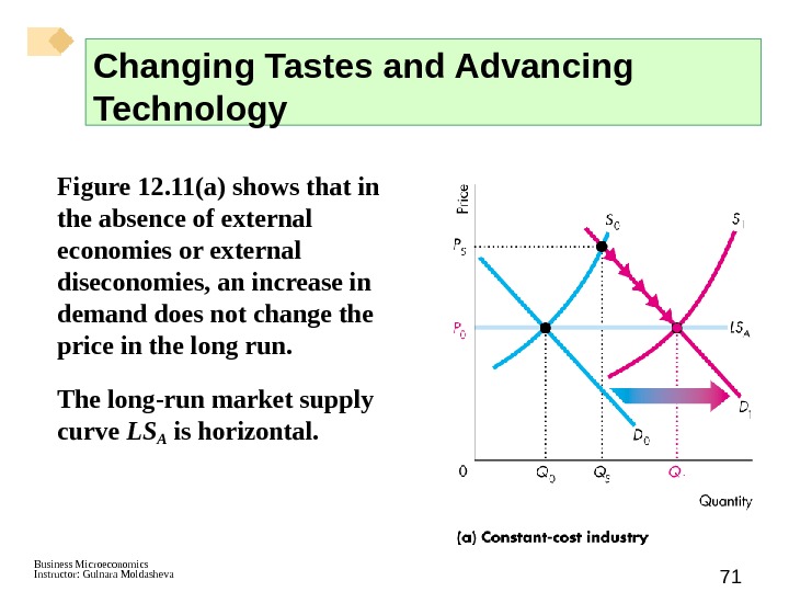
Business Microeconomics Instructor: Gulnara Moldasheva 71 Figure 12. 11(a) shows that in the absence of external economies or external diseconomies, an increase in demand does not change the price in the long run. The long-run market supply curve LSA is horizontal. Changing Tastes and Advancing Technology

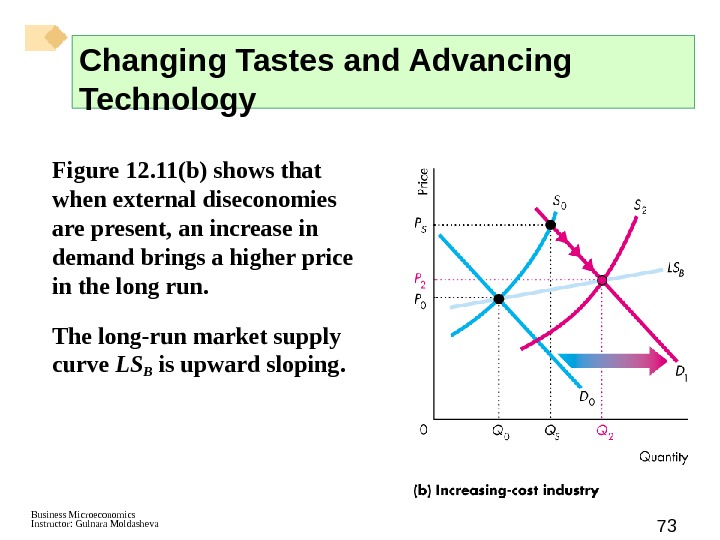
Business Microeconomics Instructor: Gulnara Moldasheva 73 Figure 12. 11(b) shows that when external diseconomies are present, an increase in demand brings a higher price in the long run. The long-run market supply curve LSB is upward sloping. Changing Tastes and Advancing Technology

Business Microeconomics Instructor: Gulnara Moldasheva 75 Figure 12. 11(c) shows that when external economies are present, an increase in demand brings a lower price in the long run. The long-run market supply curve LSC is downward sloping. Changing Tastes and Advancing Technology

Business Microeconomics Instructor: Gulnara Moldasheva 77 Technological Change New technologies are constantly discovered that lower costs. A new technology enables firms to produce at a lower average cost and a lower marginal cost— firms’ cost curves shift downward. Firms that adopt the new technology make an economic profit. Changing Tastes and Advancing Technology

Business Microeconomics Instructor: Gulnara Moldasheva 78 New-technology firms enter and old-technology firms either exit or adopt the new technology. Industry supply increases and the industry supply curve shifts rightward. The price falls and the quantity increases. Eventually, a new long-run equilibrium emerges in which all firms use the new technology, the price equals minimum average total cost, and each firm makes zero economic profit. Changing Tastes and Advancing Technology

Business Microeconomics Instructor: Gulnara Moldasheva 79 Competition and Efficiency Efficient Use of Resources are used efficiently when no one can be made better off without making someone else worse off. This situation arises when marginal social benefit equals marginal social cost.

Business Microeconomics Instructor: Gulnara Moldasheva 80 Choices, Equilibrium, and Efficiency We can describe an efficient use of resources in terms of the choices of consumers and firms coordinated in market equilibrium. Choices A consumer’s demand curve shows how the best budget allocation changes as the price of a good changes. So consumers get the most value out of their resources at all points along their demand curves. With no external benefits, the market demand curve is the marginal social benefit curve. Competition and Efficiency

Business Microeconomics Instructor: Gulnara Moldasheva 81 A competitive firm’s supply curve shows how the profit-maximizing quantity changes as the price of a good changes. So firms get the most value out of their resources at all points along their supply curves. With no external cost, the market supply curve is the marginal social cost curve. Competition and Efficiency

Business Microeconomics Instructor: Gulnara Moldasheva 82 Equilibrium and Efficiency In competitive equilibrium, resources are used efficiently— the quantity demanded equals the quantity supplied, so marginal social benefit equals marginal social cost. The gains from trade for consumers is measured by consumer surplus. The gains from trade for producers is measured by producer surplus. Total gains from trade equal total surplus. In long-run equilibrium total surplus is maximized. Competition and Efficiency

Business Microeconomics Instructor: Gulnara Moldasheva 83 Figure 12. 12 illustrates an efficient allocation of resources in a perfectly competitive market. At the market price P *, each firm is producing the quantity q *at the lowest possible long-run average total cost. Competition and Efficiency

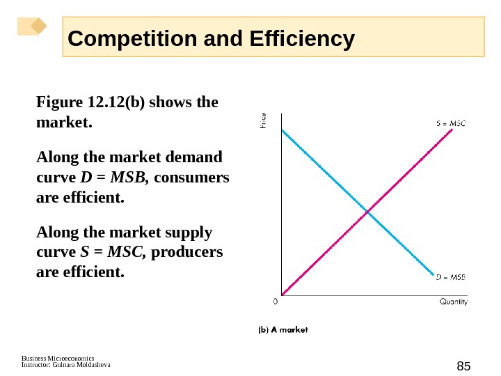
Business Microeconomics Instructor: Gulnara Moldasheva 85 Figure 12. 12(b) shows the market. Along the market demand curve D = MSB, consumers are efficient. Along the market supply curve S = MSC, producers are efficient. Competition and Efficiency

Business Microeconomics Instructor: Gulnara Moldasheva 87 The quantity Q * and price P * are the competitive equilibrium values. So competitive equilibrium is efficient. Total surplus, the sum of consumer surplus and producer surplus, is maximized. Competition and Efficiency