11. What is Econometrics? 2. Steps in Empirical

11. What is Econometrics? 2. Steps in Empirical Economic Analysis 3. Examples 4. Economic Data 5. Causality and the notion of “Ceteris Paribus”THE NATURE OF ECONOMETRICS AND ECONOMIC DAT

2 • Combination of statistical methods , economics and data to answer empirical questions in economics. 1. WHAT IS ECONOMETRICS? There are many different types of empirical questions in economics

3 • Estimation of economic relationships: — Demand supply equations; — Production functions; — Wage equations, etc. • Evaluating government policies: — Employment effects of an increase in the minimum wage; — Effects of monetary policy on inflation. • Evaluating business policies: — Estimate the optimal price and advertising expenditure for a new product; — Compare profits under two pricing policies. 1. WHAT IS ECONOMETRICS?

4 • Econometrics is relevant in virtually every branch of applied economics : finance, labor, health, industrial, macro, development, international, trade, marketing, strategy, etc. • There are two important features which distinguish Econometrics from other applications of statistics : 1. Economic data is non-experimental data. We cannot simply classify individuals or firms in an experimental group and a control group. Individuals are typically free to self-select themselves in a group (e. g. , education, occupation, product market, etc). 2. Economic models (either simple or sophisticated) are key to interpret the statistical results in econometric applications. 1. WHAT IS ECONOMETRICS?

5 • The research process in applied econometrics is not simply linear, but it has “loops”. That is, the original question and model, and even the data collection (e. g. , search for additional information/variables) can be modified after looking at preliminary econometric results. • Keeping this in mind, it is useful to describe the different steps of the research process in econometrics: 1. Formulation of the question(s) of interest. 2. Collection of data 3. Specification of the econometric model 4. Estimation, validation, hypotheses testing, prediction. 2. STEPS IN EMPIRICAL ECONOMIC ANALYSIS

6 Step 1: Empirical question(s) • Learning-by-doing (LBD) is the process by which the cost of producing a good declines with the cumulative output that the firm (or plant) has produced. • Suppose that the managers of INTEL, the CPU manufacturer, would like to measure the degree of learning-by-doing in the costs of producing a new type of CPU. • This is important for the decision of the time-path of production of the new product. • Regulators are also interested in LBD because it has implications on market structure, competition and welfare. 3. EXAMPLE: Learning-by-doing in Production Costs

7 Step 2: Collection of data • There are different of datasets that can be collected to study learning by doing. 1. Data on production costs versus data on output and inputs. 2. Data at the plant level versus aggregate data at the firm level. 3. Time series data (e. g. , a plant over several months), or cross-sectional data (e. g. , many production plants at the same period); or panel data (e. g. , many production plants over multiple periods). 3. EXAMPLE: Learning-by-doing in Production Costs

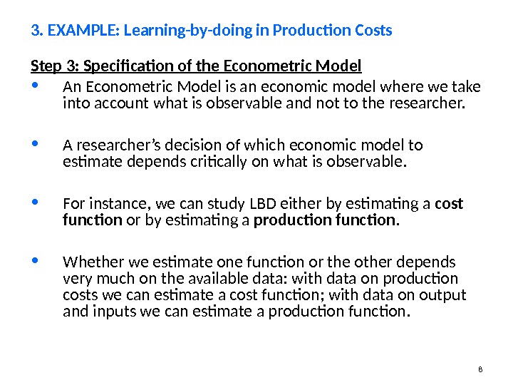
8 Step 3: Specification of the Econometric Model • An Econometric Model is an economic model where we take into account what is observable and not to the researcher. • A researcher’s decision of which economic model to estimate depends critically on what is observable. • For instance, we can study LBD either by estimating a cost function or by estimating a production function. • Whether we estimate one function or the other depends very much on the available data: with data on production costs we can estimate a cost function; with data on output and inputs we can estimate a production function. 3. EXAMPLE: Learning-by-doing in Production Costs

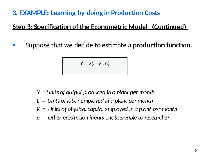
9 Step 3: Specification of the Econometric Model (Continued) • Suppose that we decide to estimate a production function. 3. EXAMPLE: Learning-by-doing in Production Costs Y = F(L , K , e ) Y = Units of output produced in a plant per month. L = Units of labor employed in a plant per month K = Units of physical capital employed in a plant per month e = Other production inputs unobservable to researcher

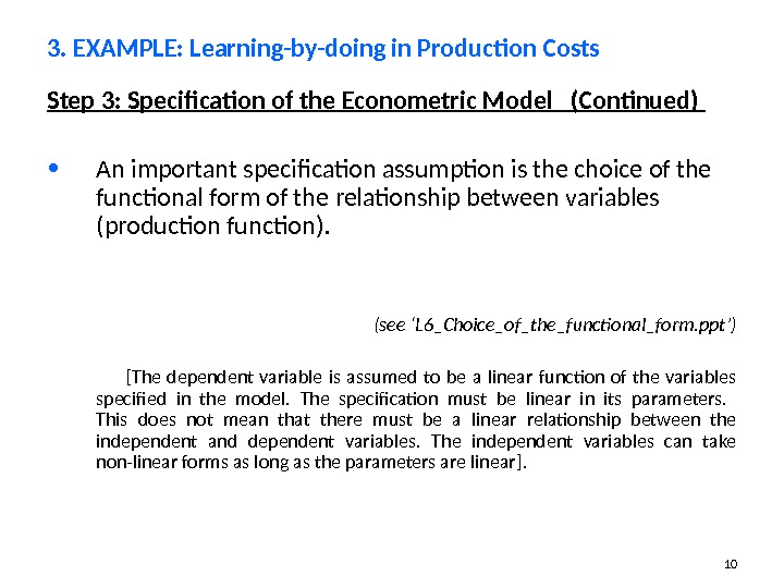
10 Step 3: Specification of the Econometric Model (Continued) • An important specification assumption is the choice of the functional form of the relationship between variables ( production function ). (see ‘L 6_Choice_of_the_functional_form. ppt’) [ The dependent variable is assumed to be a linear function of the variables specified in the model. The specification must be linear in its parameters. This does not mean that there must be a linear relationship between the independent and dependent variables. The independent variables can take non-linear forms as long as the parameters are linear ]. 3. EXAMPLE: Learning-by-doing in Production Costs

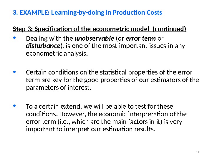
11 Step 3: Specification of the econometric model (continued) • Dealing with the unobservable (or error term or disturbance ) , is one of the most important issues in any econometric analysis. • Certain conditions on the statistical properties of the error term are key for the good properties of our estimators of the parameters of interest. • To a certain extend, we will be able to test for these conditions. However, the economic interpretation of the error term (i. e. , which are the main factors in it) is very important to interpret our estimation results. 3. EXAMPLE: Learning-by-doing in Production Costs

12 Step 4: Estimation, validation, hypotheses testing, prediction • We want to estimate the parameters β in the production function. After estimation, we have to make specification tests in order to validate some of the specification assumptions that we have made for estimation. • The results of these tests may imply a re-specification and re-estimation of the model. • Once we have a validated model, we can interpret the results from an economic point of view, make tests, and predictions. • For instance, we may be interested in testing the significance of LBD. • We may also be interested in testing constant returns to scale. Note that LBD implies that short-run and long-run returns to scale differ. 3. EXAMPLE: Learning-by-doing in Production Costs

13 • Different types of datasets have their own issues, advantages and limitations. • Some econometric methods may be valid (i. e. , have good properties) for some types of data but not for others. • We typically distinguish three types of datasets: 1. Cross-Sectional Data 2. Time Series Data 3. Panel Data 4. Economic Data

14 Cross-Sectional Data • A cross-sectional dataset is a sample of individuals, or households, or firms, or cities, or states, or countries, …, taken at a given point in time. • We often assume that these data have been obtained by random sampling. • Sometimes we do not have a random sample. 4. Economic Data

15 Time Series Data • A time series dataset consists of observations on a variable or several variables over several periods of time (days, weeks, months, years). • A key feature of time series data is that, typically, observations are correlated across time. We do not have a random sample. • This time correlation introduces very important issues in the estimation and testing of econometric models using time series data. • Seasonality is other common feature in many weekly, monthly or quarterly time series data. 4. Economic Data

16 Pooled cross sections • Suppose that we have a sequence of cross sections of the same variables and from the same population at years 1990, 1991, 1992, … and 2005. That is called a pooled cross-sectional data. • It is useful data to analyze the evolution over time of the cross-sectional distribution of variables such as individual wages, household income, firms’ investments, etc. • We should distinguish pooled cross-sections from panel data. • In pooled cross sections we do not follow the same individuals over time. Every period we have a new random sample of individuals. 4. Economic Data

17 Panel Data • In panel data we have a group of individuals (or households, firms, countries, …) who are observed at several points in time. That is, we have time series data for each individual in the sample. • The key feature of panel data that distinguishes them from pooled cross sections is that the same individuals are followed over a given period of time. 4. Economic Data

18 • Most empirical questions in economics are associated to the identification of CAUSAL EFFECTS. • The notion of ceteris paribus (i. e. , “other factors being equal”) plays an important role in the analysis of causality. • Consider the example of LBD in the production of micro-chips. • To identify the effect of LBD, ideally, we would like to observe two production plants which are identical in all its inputs (both observable and unobservable to the researcher). 5. Causality and the notion of “Ceteris Paribus”

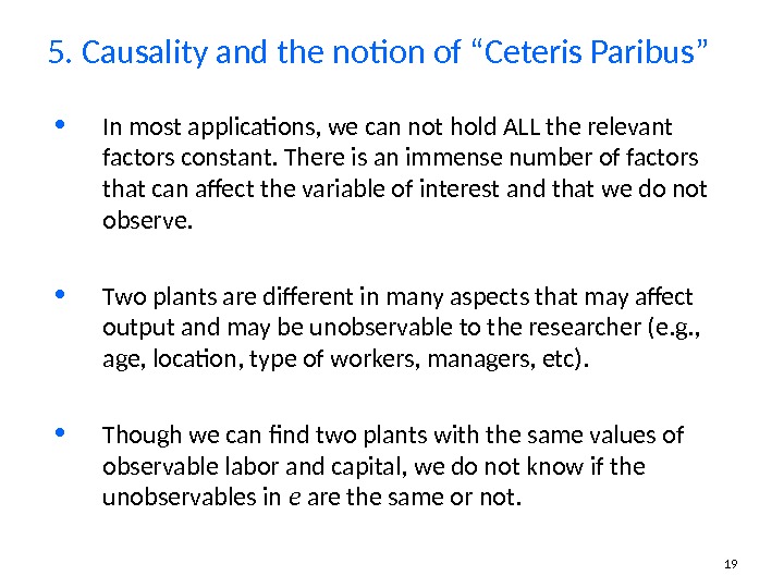
19 • In most applications, we can not hold ALL the relevant factors constant. There is an immense number of factors that can affect the variable of interest and that we do not observe. • Two plants are different in many aspects that may affect output and may be unobservable to the researcher (e. g. , age, location, type of workers, managers, etc). • Though we can find two plants with the same values of observable labor and capital, we do not know if the unobservables in e are the same or not. 5. Causality and the notion of “Ceteris Paribus”

20 • Does it mean that we cannot identify causal effects? • Not necessarily. In fact, there are cases where we can identify causal effects using careful econometric analysis. • What we need to identify causal effects is to hold constant all the relevant factors which are not independent of the causal variable under study. • We do not have to hold constant those factors which are independent of the causal variable. 5. Causality and the notion of “Ceteris Paribus”

• We make two assumptions about the explanatory variables: 1. The explanatory variables are not random variables • We are assuming that the values of the explanatory variables are known to us prior to our observing the values of the dependent variable

• We make two assumptions about the explanatory variables (Continued) : 2. Any one of the explanatory variables is not an exact linear function of the others • This assumption is equivalent to assuming that no variable is redundant • If this assumption is violated – a condition called exact collinearity — the least squares procedure fails

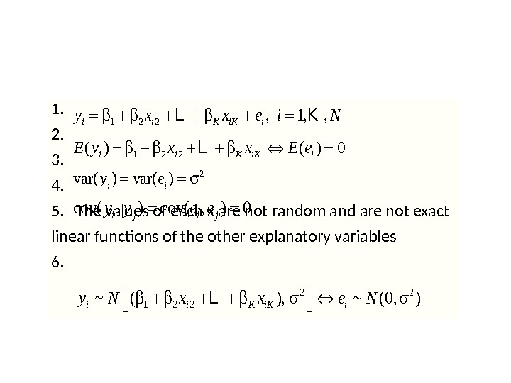
1. 2. 3. 4. 5. The values of each x are not random and are not exact linear functions of the other explanatory variables 6. 1 2 2, 1, , i i K iy x x e i N L K 1 2 2( ) 0 i i K i. E y x x E e L 2 var( )i iy e cov( , ) 0 i j i jy y e e 2 2 1 2 2~ ( ), ~ (0, )i i K iy N x x e N L

Steps in building and using an econometric model STEP 1: Decide what is the “Dependent Variable”, i. e. the variable whose observed values are to be explained: Y t or Y i NOTE: the subscript is used to emphasise that the model will seek to explain the values of the dependent variable that have been observed at particular dates (time series data Y t ) or at particular objects (cross-sectional data Y i )

Steps in building and using an econometric model STEP 2 : Decide, on the basis of economic theory, what are the appropriate potential explanatory variables for the given dependent variable. Definitely in the model: X 1 t , X 2 t , … X kt or X 1 i , X 2 i , … X ki β 0 , β 1 , β 2 , …, β k , ε t or ε i — An unobservable error term, representing the existence of other unknown causal factors whose random fluctuations cause the dependent variable to not do exactly what is expected on the basis of the known explanatory variables alone.

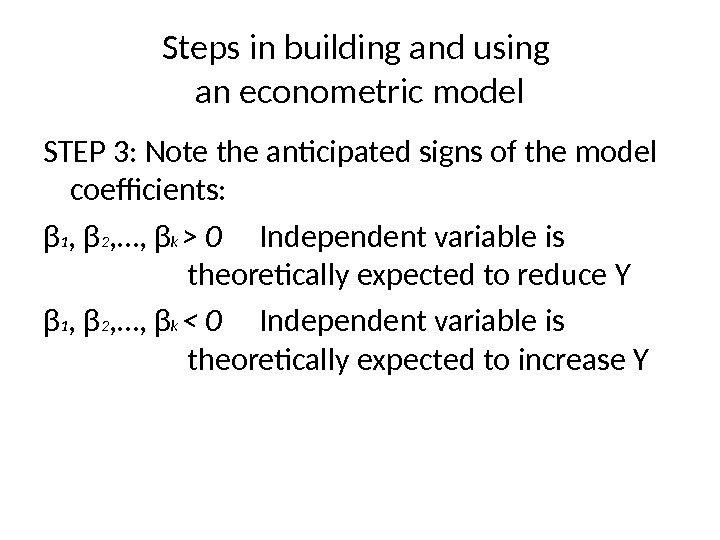
Steps in building and using an econometric model STEP 3 : Note the anticipated signs of the model coefficients: β 1 , β 2 , …, β k > 0 Independent variable is theoretically expected to reduce Y β 1 , β 2 , …, β k < 0 Independent variable is theoretically expected to increas e Y

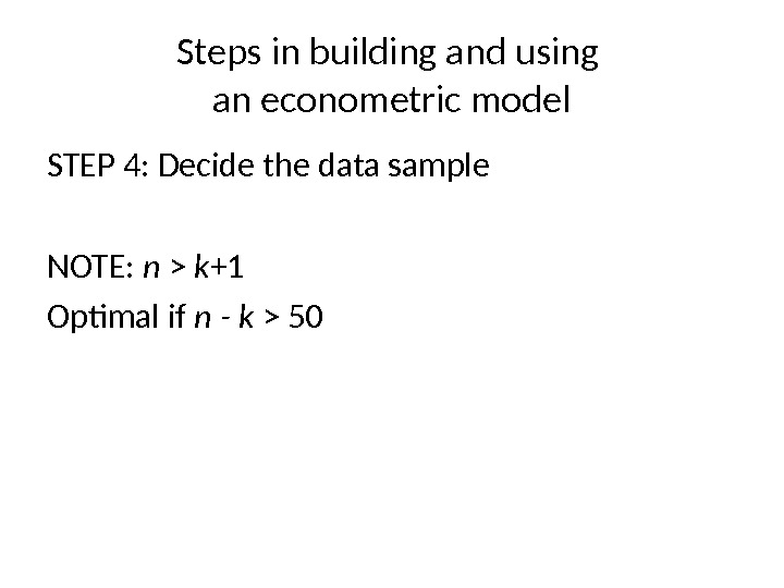
Steps in building and using an econometric model STEP 4 : Decide the data sample NOTE: n > k +1 Optimal if n — k >

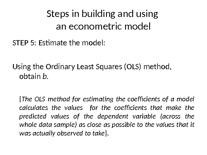
Steps in building and using an econometric model STEP 5 : Estimate the m odel: Using the Ordinary Least Squares (OLS) method, obtain b. [ The OLS method for estimating the coefficients of a model calculates the values for the coefficients that make the predicted values of the dependent variable (across the whole data sample) as close as possible to the values that it was actually observed to take ].

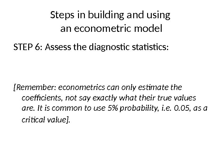
Steps in building and using an econometric model STEP 6 : Assess the diagnostic statistics : [Remember: econometrics can only estimate the coefficients, not say exactly what their true values are. It is common to use 5% probability, i. e. 0. 05, as a critical value ].

Steps in building and using an econometric model STEP 7 : Interpret the results : [Remember: econometrics can only estimate the coefficients, not say exactly what their true values are. It is common to use 5% probability, i. e. 0. 05, as a critical value ]. © Vince Daly & Kingston University, October 6, 2009 This work is licenced under a Creative Commons Licence

NOTE: The results may imply a re-specification and re-estimation of the model …