1 Output and Costs CHAPTER 11 2 After

1 Output and Costs CHAPTER 11

2 After studying this chapter you will be able to Distinguish between the short run and the long run Explain the relationship between a firm’s output and labor employed in the short run Explain the relationship between a firm’s output and costs in the short run and derive a firm’s short-run cost curves Explain the relationship between a firm’s output and costs in the long run and derive a firm’s long-run average cost curve

3 Survival of the Fittest Size does not guarantee survival in business. Even large firms can disappear or get eaten up by other firms. Millions of small firms close down each year. What does a firm have to do to be a survivor? All firm have to decided how much to produce and how to produce it. How do firms make these decisions? This chapter studies a firm’s production possibilities and costs of production.

4 Decision Time Frames The firm makes many decisions to achieve its main objective: profit maximization. Some decisions are critical to the survival of the firm. Some decisions are irreversible (or very costly to reverse). Other decisions are easily reversed and are less critical to the survival of the firm, but still influence profit. All decisions can be placed in two time frames: The short run The long run

5 Decision Time Frames The Short Run The short run is a time frame in which the quantity of one or more resources used in production is fixed. For most firms, the capital, called the firm’s plant, is fixed in the short run. Other resources used by the firm (such as labor, raw materials, and energy) can be changed in the short run. Short-run decisions are easily reversed.

6 Decision Time Frames The Long Run The long run is a time frame in which the quantities of all resources—including the plant size—can be varied. Long-run decisions are not easily reversed. A sunk cost is a cost incurred by the firm and cannot be changed. If a firm’s plant has no resale value, the amount paid for it is a sunk cost. Sunk costs are irrelevant to a firm’s decisions.

7 Short-Run Technology Constraint To increase output in the short run, a firm must increase the amount of labor employed. Three concepts describe the relationship between output and the quantity of labor employed: 1. Total product 2. Marginal product 3. Average product

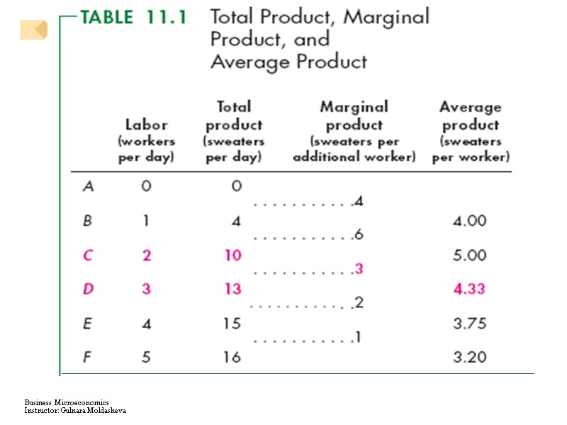
8 Short-Run Technology Constraint Product Schedules Total product is the total output produced in a given period. The marginal product of labor is the change in total product that results from a one-unit increase in the quantity of labor employed, with all other inputs remaining the same. The average product of labor is equal to total product divided by the quantity of labor employed. Table 11.1 shows a firm’s product schedules.

9 Short-Run Technology Constraint

11 Short-Run Technology Constraint Product Curves Product curves are graphs of the three product concepts that show how total product, marginal product, and average product change as the quantity of labor employed changes.

12 Short-Run Technology Constraint Total Product Curve Figure 11.1 shows a total product curve. The total product curve shows how total product changes with the quantity of labor employed.

13

14 Short-Run Technology Constraint The total product curve is similar to the PPF. It separates attainable output levels from unattainable output levels in the short run.

15 Short-Run Technology Constraint Marginal Product Curve Figure 11.2 shows the marginal product of labor curve and how the marginal product curve relates to the total product curve. The first worker hired produces 4 units of output.

16

17 Short-Run Technology Constraint The second worker hired produces 6 units of output and total product becomes 10 units. The third worker hired produces 3 units of output and total product becomes 13 units. And so on.

18 Short-Run Technology Constraint The height of each bar measures the marginal product of labor. For example, when labor increases from 2 to 3, total product increases from 10 to 13, so the marginal product of the third worker is 3 units of output.

19 Short-Run Technology Constraint To make a graph of the marginal product of labor, we can stack the bars in the previous graph side by side. The marginal product of labor curve passes through the mid-points of these bars.

20

21 Short-Run Technology Constraint Almost all production processes are like the one shown here and have: Increasing marginal returns initially Diminishing marginal returns eventually

22 Short-Run Technology Constraint Increasing Marginal Returns Initially When the marginal product of a worker exceeds the marginal product of the previous worker, the marginal product of labor increases and the firm experiences increasing marginal returns.

23 Short-Run Technology Constraint Diminishing Marginal Returns Eventually When the marginal product of a worker is less than the marginal product of the previous worker, the marginal product of labor decreases. The firm experiences diminishing marginal returns.

24 Short-Run Technology Constraint Increasing marginal returns arise from increased specialization and division of labor. Diminishing marginal returns arises from the fact that employing additional units of labor means each worker has less access to capital and less space in which to work. Diminishing marginal returns are so pervasive that they are elevated to the status of a “law.” The law of diminishing returns states that as a firm uses more of a variable input with a given quantity of fixed inputs, the marginal product of the variable input eventually diminishes.

25 Short-Run Technology Constraint Average Product Curve Figure 10.3 shows the average product curve and its relationship with the marginal product curve. When marginal product exceeds average product, average product increases.

26

27 Short-Run Technology Constraint When marginal product is below average product, average product decreases. When marginal product equals average product, average product is at its maximum.

28 Short-Run Technology Constraint Marginal Grade and Grade Point Average The relationship between a student’s marginal class grade and her or his grade point average (GPA) is similar to that between marginal product and average product. If a student’s next class grade is higher (lower) than the student’s GPA, this marginal grade will pull the student’s GPA (average grade) up (down). If the next class grade is the same as the GPA, the GPA remains unchanged.

29 Short-Run Cost To produce more output in the short run, the firm must employ more labor, which means that it must increase its costs. We describe the way a firm’s costs change as total product changes by using three cost concepts and three types of cost curve: Total cost Marginal cost Average cost

30 Short-Run Cost Total Cost A firm’s total cost (TC) is the cost of all resources used. Total fixed cost (TFC) is the cost of the firm’s fixed inputs. Fixed costs do not change with output (Any cost that does not depend on the firm’s level of output). These costs are incurred even if the firm is producing nothing. There are no fixed costs in the long run. Total variable cost (TVC) is the cost of the firm’s variable inputs. Variable costs do change with output. Total cost equals total fixed cost plus total variable cost. That is: TC = TFC + TVC

31 Short-Run Cost

32 Short-Run Cost Total fixed costs (TFC) or overhead The total of all costs that do not change with output, even if output is zero. Total Fixed Cost (TFC) FIXED COSTS Firms have no control over fixed costs in the short run. For this reason, fixed costs are sometimes called sunk costs.

33 COSTS IN THE SHORT RUN sunk costs Another name for fixed costs in the short run because firms have no choice but to pay them. average fixed cost (AFC) Total fixed cost divided by the number of units of output; a per-unit measure of fixed costs. Average Fixed Cost (AFC)

34 COSTS IN THE SHORT RUN spreading overhead The process of dividing total fixed costs by more units of output. Average fixed cost declines as quantity rises. FIGURE 10.2 Short-Run Fixed Cost (Total and Average) of a Hypothetical Firm

35 Short-Run Cost Figure 10.4 shows a firm’s total cost curves. Total fixed cost is the same at each output level. Total variable cost increases as output increases. Total cost, which is the sum of TFC and TVC also increases as output increases.

36

37 Short-Run Cost The total variable cost curve gets its shape from the total product curve. Notice that the TP curve becomes steeper at low output levels and then less steep at high output levels. In contrast, the TVC curve becomes less steep at low output levels and steeper at high output levels.

38

39 COSTS IN THE SHORT RUN

40 COSTS IN THE SHORT RUN The total variable cost curve embodies information about both factor, or input, prices and technology. It shows the cost of production using the best available technique at each output level given current factor prices. FIGURE 10.3 Total Variable Cost Curve

41 Short-Run Cost To see the relationship between the TVC curve and the TP curve, lets look again at the TP curve. But let us add a second x-axis to measure total variable cost. 1 worker costs $25; 2 workers cost $50: and so on, so the two x-axes line up.

42

43 Short-Run Cost We can replace the quantity of labor on the x-axis with total variable cost. When we do that, we must change the name of the curve. It is now the TVC curve. But it is graphed with cost on the x-axis and output on the y-axis.

44

45 Short-Run Cost Redraw the graph with cost on the y-axis and output on the x-axis, and you’ve got the TVC curve drawn the usual way. Put the TFC curve back in the figure, and add TFC to TVC, and you’ve got the TC curve.

46

47 Short-Run Cost Marginal Cost Marginal cost (MC) is the increase in total cost that results from a one-unit increase in total product. Over the output range with increasing marginal returns, marginal cost falls as output increases. Over the output range with diminishing marginal returns, marginal cost rises as output increases.

48 COSTS IN THE SHORT RUN Although the easiest way to derive marginal cost is to look at total variable cost and subtract, do not lose sight of the fact that when a firm increases its output level, it hires or demands more inputs. Marginal cost measures the additional cost of inputs required to produce each successive unit of output. Marginal cost (MC) The increase in total cost that results from producing one more unit of output. Marginal costs reflect changes in variable costs.

49 COSTS IN THE SHORT RUN The Shape of the Marginal Cost Curve in the Short Run FIGURE 10.4 Declining Marginal Product Implies That Marginal Cost Will Eventually Rise with Output

50 Short-Run Cost Average Cost Average cost measures can be derived from each of the total cost measures: Average fixed cost (AFC) is total fixed cost per unit of output. Average variable cost (AVC) is total variable cost per unit of output. Average total cost (ATC) is total cost per unit of output. ATC = AFC + AVC.

51 Short-Run Cost: Table to Figure 11.5

52 Short-Run Cost Figure 10.5 shows the MC, AFC, AVC, and ATC curves. The AFC curve shows that average fixed cost falls as output increases. The AVC curve is U-shaped. As output increases, average variable cost falls to a minimum and then increases.

53

54 Short-Run Cost The ATC curve is also U-shaped. The MC curve is very special. Where AVC is falling, MC is below AVC. Where AVC is rising, MC is above AVC. At the minimum AVC, MC equals AVC.

55

56 Short-Run Cost Similarly, where ATC is falling, MC is below ATC. Where ATC is rising, MC is above ATC. At the minimum ATC, MC equals ATC.

57

58 Short-Run Cost Why the Average Total Cost Curve Is U-Shaped The AVC curve is U-shaped because: Initially, marginal product exceeds average product, which brings rising average product and falling AVC. Eventually, marginal product falls below average product, which brings falling average product and rising AVC. The ATC curve is U-shaped for the same reasons. In addition, ATC falls at low output levels because AFC is falling steeply.

59 Short-Run Cost Cost Curves and Product Curves The shapes of a firm’s cost curves are determined by the technology it uses: MC is at its minimum at the same output level at which marginal product is at its maximum. When marginal product is rising, marginal cost is falling. AVC is at its minimum at the same output level at which average product is at its maximum. When average product is rising, average variable cost is falling.

60 Short-Run Cost Figure 10.6 shows these relationships.

61

62 COSTS IN THE SHORT RUN Marginal cost is the cost of one additional unit. Average variable cost is the total variable cost divided by the total number of units produced.

63 Short-Run Cost Shifts in Cost Curves The position of a firm’s cost curves depend on two factors: Technology Prices of factors of production

64 Short-Run Cost Technology Technological change influences both the productivity curves and the cost curves. An increase in productivity shifts the average and marginal product curves upward and the average and marginal cost curves downward. If a technological advance brings more capital and less labor into use, fixed costs increase and variable costs decrease. In this case, average total cost increases at low output levels and decreases at high output levels.

65 Short-Run Cost Prices of Factors of Production An increase in the price of a factor of production increases costs and shifts the cost curves. An increase in a fixed cost shifts the total cost (TC ) and average total cost (ATC ) curves upward but does not shift the marginal cost (MC ) curve. An increase in a variable cost shifts the total cost (TC ), average total cost (ATC ), and marginal cost (MC ) curves upward.

66 SHORT-RUN COSTS: A REVIEW

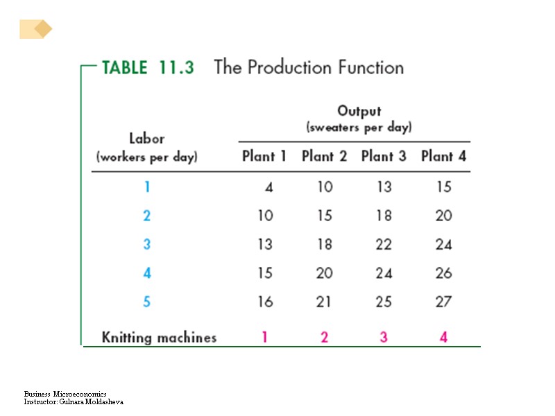
67 Long-Run Cost In the long run, all inputs are variable and all costs are variable. The Production Function The behavior of long-run cost depends upon the firm’s production function, which is the relationship between the maximum output attainable and the quantities of both capital and labor. Table 11.3 shows a production function.

Long-Run Cost Table 11.3 shows a firm’s production function. As the size of the plant increases, the output that a given quantity of labor can produce increases. But as the quantity of labor increases, diminishing returns occur for each plant.

69

71 Long-Run Cost Diminishing Marginal Product of Capital The marginal product of capital is the increase in output resulting from a one-unit increase in the amount of capital employed, holding constant the amount of labor employed. A firm’s production function exhibits diminishing marginal returns to labor (for a given plant size) as well as diminishing marginal returns to capital (for a quantity of labor). For each plant size, diminishing marginal product of labor creates a set of short run, U-shaped costs curves for MC, AVC, and ATC.

72 Long-Run Cost Short-Run Cost and Long-Run Cost The average cost of producing a given output varies and depends on the firm’s plant size. The larger the plant size, the greater is the output at which ATC is at a minimum. Cindy has 4 different plant sizes: 1, 2, 3, or 4 knitting machines. Each plant has a short-run ATC curve. The firm can compare the ATC for each given output at different plant sizes.

73 Long-Run Cost

74

75 Long-Run Cost

76 Long-Run Cost

77 Long-Run Cost

78 Long-Run Cost The long-run average cost curve is made up from the lowest ATC for each output level. So, we want to decide which plant has the lowest cost for producing each output level. Let’s find the least-cost way of producing a given output level. Suppose that Cindy wants to produce 13 sweaters a day.

79 Long-Run Cost

80

81 Long-Run Cost

82 Long-Run Cost

83 Long-Run Cost

84 Long-Run Cost

85 Long-Run Cost Long-Run Average Cost Curve The long-run average cost curve is the relationship between the lowest attainable average total cost and output when both the plant size and labor are varied. The long-run average cost curve is a planning curve that tells the firm the plant size that minimizes the cost of producing a given output range. Once the firm has chosen that plant size, it incurs the costs that correspond to the ATC curve for that plant.

86 Long-Run Cost Figure 10.8 illustrates the long-run average cost (LRAC) curve.

87

88 Long-Run Cost Economies and Diseconomies of Scale Economies of scale are features of a firm’s technology that lead to falling long-run average cost as output increases. Diseconomies of scale are features of a firm’s technology that lead to rising long-run average cost as output increases. Constant returns to scale are features of a firm’s technology that lead to constant long-run average cost as output increases.

89 The Scale of Production Dollars Quantity Long-Run Average Cost Optimal Plant Size

90 Long-Run Cost Figure 10.8 illustrates economies and diseconomies of scale.

91

92 Long-Run Cost Minimum Efficient Scale A firm experiences economies of scale up to some output level. Beyond that output level, it moves into constant returns to scale or diseconomies of scale. Minimum efficient scale is the smallest quantity of output at which the long-run average cost reaches its lowest level. If the long-run average cost curve is U-shaped, the minimum point identifies the minimum efficient scale output level.

93 average fixed cost (AFC) average total cost (ATC) average variable cost (AVC) fixed cost marginal cost (MC) marginal revenue (MR) spreading overhead sunk costs total cost (TC) total fixed costs (TFC), or overhead total revenue (TR) total variable cost (TVC) REVIEW TERMS AND CONCEPTS total variable cost curve variable cost 1. TC = TFC + TVC 2. AFC = TFC/q 3. Slope of TVC = MC 4. AVC = TVC/q 5. ATC = TC/q = AFC + AVC 6. TR = P x q 7. Profit-maximizing level of output for all firms: MR = MC 8. Profit-maximizing level of output for perfectly competitive firms: P = MC